How do electric fields differ from magnetic fields?
Electric and magnetic fields are two sides of the same coin—the electromagnetic force—but they possess distinct origins, behaviors, and effects on matter that make differentiating them essential for physics and engineering. While we frequently discuss them together, recognizing their individual characteristics is the first step toward grasping the full scope of electromagnetism.
# Field Genesis
The fundamental difference between these two fields lies in what generates them. An electric field () arises directly from the presence of electric charge, irrespective of its state of motion. Any static, stationary charge—positive or negative—will create an electric field extending outward from it into space. This field strength decreases based on the square of the distance from the charge.
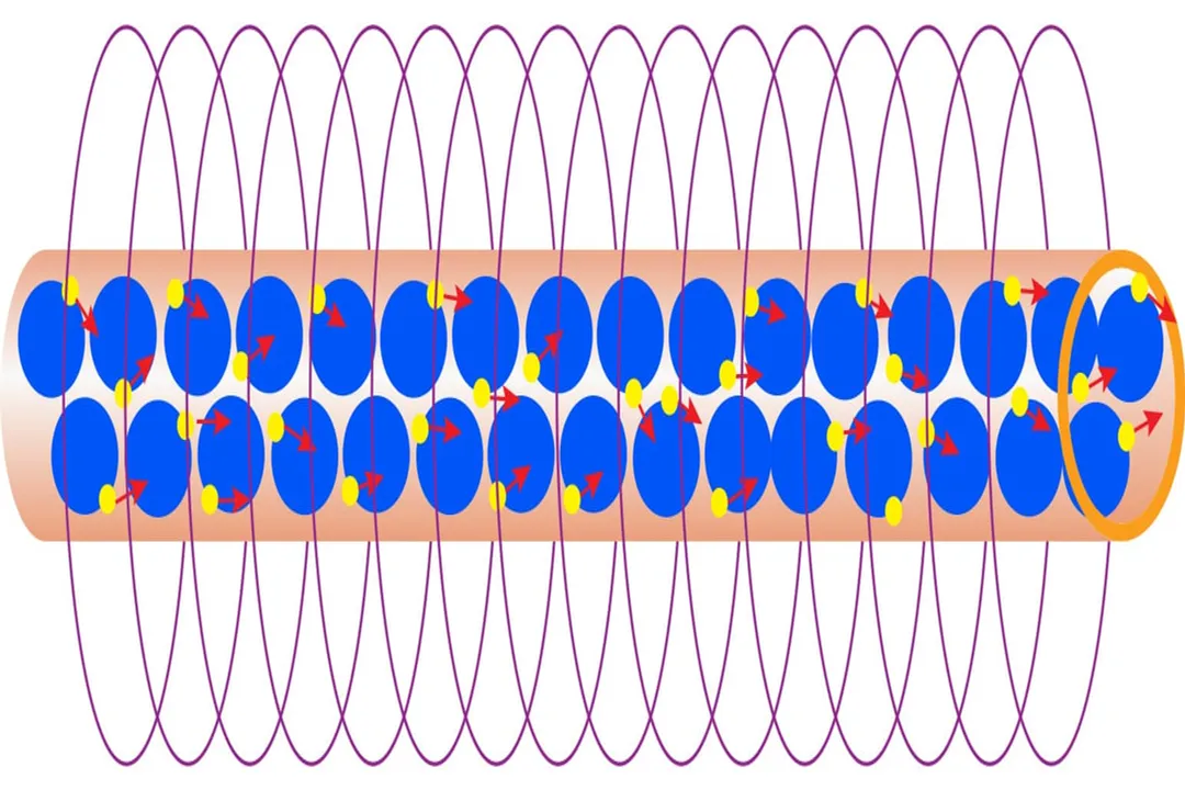
Magnetic fields (), conversely, are created exclusively by moving electric charges. This movement is what we typically define as an electric current. A stationary charge generates zero magnetic field. If a wire carrying a current is switched off, the magnetic field surrounding it collapses immediately, because the source (the moving charge) has ceased its motion. This dependency on velocity is a primary differentiator.
# Force Action
The manner in which these fields interact with a charged particle further illustrates their differences, particularly concerning the particle's velocity.
The electric force experienced by a charge () is straightforward: . This force acts directly along the path of the electric field lines, pushing positive charges in the direction of and negative charges opposite to it. Crucially, this force is exerted whether the charge is moving or completely stationary.
The magnetic force is significantly more complicated due to its dependence on velocity (): . This equation, involving a vector cross product, dictates two critical points:
- A charge that is not moving () experiences absolutely no magnetic force, even if it is immersed in a powerful magnetic field.
- The resulting force is always perpendicular to both the direction of motion () and the magnetic field direction (). This perpendicular relationship means a magnetic field can change the direction of a moving charge's velocity, but it can never do work to change its speed.

# Field Lines Shape
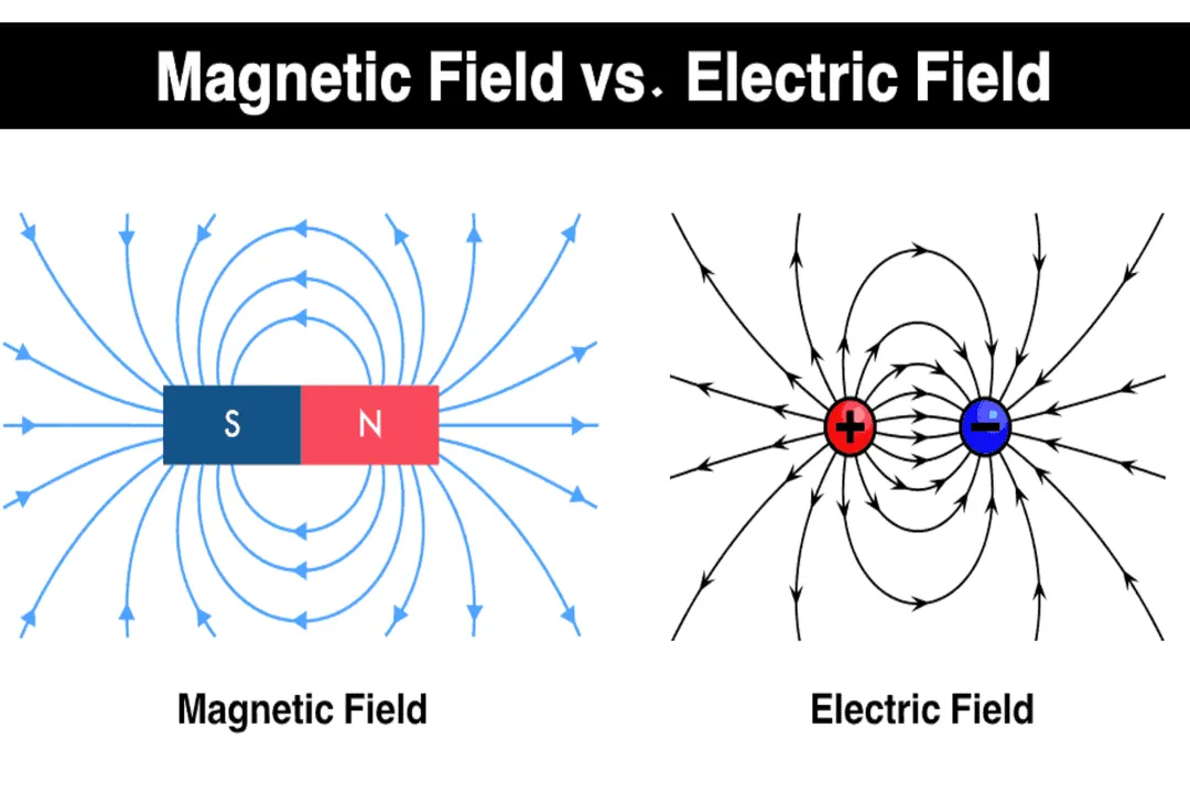
Visualizing these fields through their characteristic lines reveals a topological contrast rooted in the absence or presence of magnetic monopoles.
Electric field lines are characterized by having definite start and end points. They originate on positive charges and terminate on negative charges. Because of this, electric fields are often described as having sources and sinks.
Magnetic field lines are fundamentally different; they never begin or end. They always form complete, continuous, closed loops. If you take a bar magnet and cut it in half, you do not isolate the north pole from the south pole; instead, you create two smaller magnets, each having both poles. This persistent loop structure is a direct consequence of the empirical observation that isolated magnetic monopoles do not exist.
# Relativity View
The deep, underlying connection between electric and magnetic fields becomes apparent when viewed through the lens of special relativity. What one observer measures as purely an electric field might be measured by a second observer, moving relative to the first, as a combination of both an electric field and a magnetic field.
Imagine a charged particle moving parallel to a wire carrying a steady current. The current creates a magnetic field, which exerts a force on the moving particle. Now, switch to the particle's own reference frame. From its perspective, it is stationary, so the magnetic force must be zero. However, physics dictates that some force must still act on it. This apparent force is reconciled because the Lorentz transformation equations, which govern how space and time change between reference frames, transform the charge densities along the wire, creating a net electric field in the moving frame that accounts for the force previously attributed to magnetism. This transformation confirms that and are not truly independent entities but rather components of a single structure, the electromagnetic field tensor.

# Field Dynamics
Another key divergence relates to their sustainability in a static configuration. As noted, a static charge produces a static electric field that remains constant over time.
Magnetic fields, however, tend to be dynamic unless sustained by a constant direct current (DC). The laws governing how these fields interact when changing are what create wave propagation. Faraday's Law states that a time-varying magnetic field induces a circulating electric field. Conversely, Ampère's Law (with Maxwell's addition) states that a time-varying electric field induces a magnetic field. This mutual induction is the mechanism by which light—an electromagnetic wave—propagates through a vacuum, with the oscillating electric and magnetic fields continuously regenerating one another as they travel outward from the source. A static field does not radiate; only changing fields do.
# Practical Measures
In practical applications, the way engineers measure and mitigate these fields varies based on their source and behavior. Electric field strength is typically quantified by the potential difference per unit distance, often measured in Volts per meter (). Magnetic field strength is often measured using units like Tesla () or Gauss ().
The geometry that minimizes the static electric field—often achieved by grounding or shielding metallic enclosures to drain static charge away—is not necessarily the geometry that minimizes the magnetic field, which is generally controlled by loop area and current magnitude.
| Feature | Electric Field () | Magnetic Field () |
|---|---|---|
| Source | Stationary or moving electric charge () | Moving electric charge (current, ) |
| Force on Charge () | ; independent of velocity | ; zero if |
| Force Direction | Parallel/Anti-parallel to | Perpendicular to both and |
| Field Lines | Originate on positive charges, terminate on negative charges | Always form closed loops; no magnetic monopoles exist |
| Static State | Can exist statically (e.g., stored charge) | Requires continuous current or a changing field to persist |
When dealing with printed circuit boards (PCBs) carrying high-frequency signals, designers must actively manage both field types simultaneously. The static electric field coupling between adjacent signal traces leads to capacitive crosstalk, where energy transfers based on the proximity and the voltage difference. In contrast, the time-varying magnetic field coupling leads to inductive crosstalk, where energy transfer depends on the current flow and the mutual inductance between the traces. A long, straight trace carrying a rapidly alternating current will produce a strong, propagating magnetic field component, whereas a capacitor holding a stable DC voltage only produces an electric field component. Effective shielding requires understanding which mechanism—electric or magnetic—dominates the potential interference in that specific application scenario.
Related Questions
#Citations
Electric Field vs Magnetic Field : r/AskPhysics
Can someone please explain magnetic vs electric fields?
What's the difference between an electric and a magnetic ...
Similarities between magnetic fields and electric fields
Magnetic Field vs Electric Field
Electric Field vs Magnetic Field - Difference and Comparison
Difference between Electric Field and Magnetic Field
What are Electric and Magnetic Fields?
What are the differences between a magnetic and an ...