What defines a normal distribution?

The concept often surfaces in discussions about statistics, data analysis, and even finance, describing a specific, highly recognizable pattern found throughout the natural and social worlds. This pattern, known mathematically as the Gaussian distribution or the normal distribution, is a continuous probability distribution characterized by a unique, symmetric shape that resembles a bell. ^[1][4][6] When you plot the data points from many natural phenomena—such as the height of adult humans, measurement errors in a lab, or test scores—they tend to cluster around a central value, tapering off evenly in both directions. ^[1][3][5]

# Bell Shape

Visually, the defining feature is the bell curve. ^[3][4] This shape means the curve is highest exactly in the middle, corresponding to the most frequent observation. ^[2] As you move away from this peak in either the positive or negative direction, the frequency of observations decreases. ^[1] The curve is perfectly balanced; the left side is a mirror image of the right side. ^[1][3] Although the tails of the distribution theoretically extend infinitely in both directions, they approach, but never quite touch, the horizontal axis. ^[1][6] This indicates that while extreme values are possible, they become increasingly rare the further they deviate from the center. ^[6]

# Key Parameters

What truly defines a normal distribution, separating it from all other potential shapes, are just two measurable characteristics: the mean ($\mu \backslash mu$) and the standard deviation ($\sigma \backslash sigma$). ^[1][3][4][6] These two numbers entirely dictate the location and spread of the entire curve. ^[9]

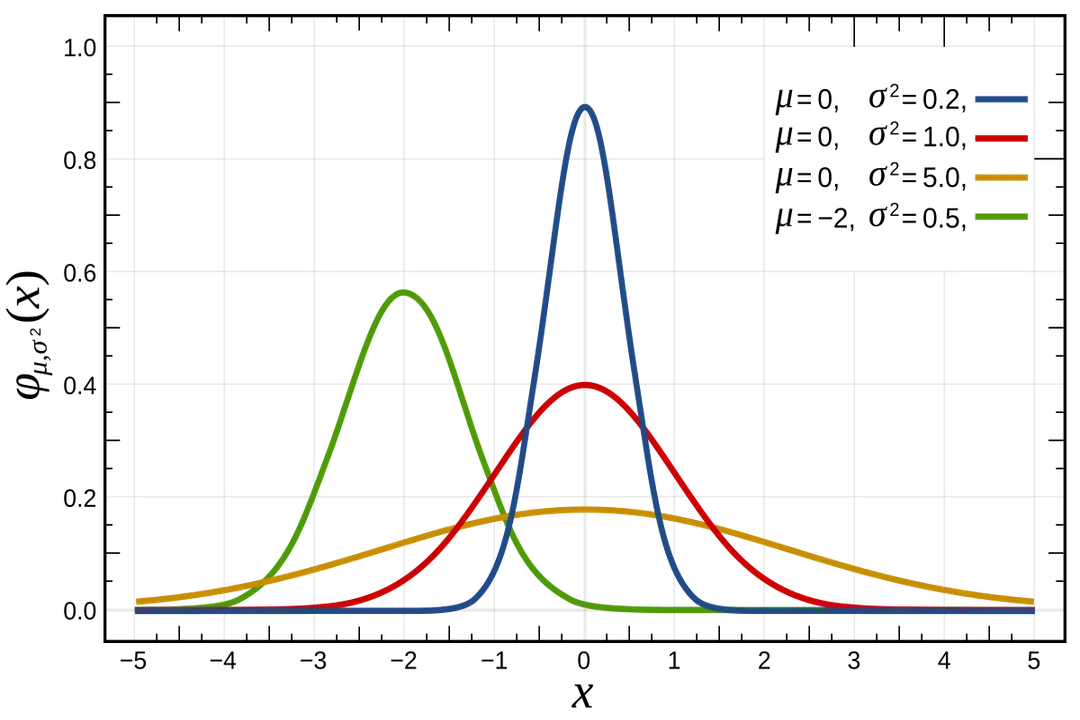
The mean ($\mu \backslash mu$), often represented by the Greek letter mu, sets the center of the distribution. ^[1][3] It is the exact point where the peak of the bell lies. ^[2] If you change the mean, the entire curve shifts left or right along the horizontal axis without changing its shape. ^[4]

The standard deviation ($\sigma \backslash sigma$), or sigma, controls the spread or dispersion of the data. ^[4][9] A small standard deviation means that most of the data points are tightly clustered around the mean, resulting in a tall, narrow, and steep bell shape. ^[1] Conversely, a large standard deviation indicates that the data is much more spread out, leading to a short, wide, and shallow bell shape. ^[9]

Consider two groups of students taking the same exam. Group A has a mean score of 80 with a standard deviation of 3 ($\mu =80,\sigma =3\backslash mu=80,\; \backslash sigma=3$). Group B also has a mean score of 80, but their standard deviation is 15 ($\mu =80,\sigma =15\backslash mu=80,\; \backslash sigma=15$). For Group A, almost everyone scored very close to 80. For Group B, while the average is still 80, there will be a significant number of students scoring much lower (e.g., 65) and much higher (e.g., 95). ^[1] The difference in $\sigma \backslash sigma$ dictates how predictable the outcome is for any single individual within that group.

Parameter	Symbol	Function	Effect on Curve
Mean	$\mu \backslash mu$	Determines the central location	Shifts the curve left or right
Standard Deviation	$\sigma \backslash sigma$	Measures data spread/variability	Changes the height and width of the curve [1][9]

# Symmetry Properties

A hallmark of the normal distribution is its perfect symmetry around the mean. ^[2] Because of this balance, the three primary measures of central tendency—the mean, the median, and the mode—are identical when the data follows this distribution. ^[2][3] The mode is the most frequent value (the peak), the median is the middle value (the 50th percentile), and the mean is the arithmetic average. ^[2] In a skewed distribution, these three points would separate; however, in the normal distribution, they all converge at the center point $\mu \backslash mu$. ^[3]

This symmetry is what allows statisticians to make definitive statements about where data should fall relative to the center. If a value is a certain distance above the mean, the probability of observing a value that same distance below the mean is exactly equal. ^[1]

# Empirical Rule

This symmetry and known spread allow us to use a powerful shortcut known as the Empirical Rule, often called the 68-95-99.7 Rule. ^[3][8] This rule is essential because it provides concrete percentages for how observations are distributed based only on the standard deviation. ^[4]

The rule states that for any dataset that is normally distributed:

1. Approximately 68% of the data falls within one standard deviation ($\pm 1\sigma \backslash pm\; 1\backslash sigma$) of the mean ($\mu \backslash mu$). ^[1][8]
2. Approximately 95% of the data falls within two standard deviations ($\pm 2\sigma \backslash pm\; 2\backslash sigma$) of the mean. ^[4][8]
3. Approximately 99.7% of the data falls within three standard deviations ($\pm 3\sigma \backslash pm\; 3\backslash sigma$) of the mean. ^[3][8]

This means that if you measure the weights of thousands of apples grown from a single tree variety, you can confidently state that virtually all of them (99.7%) will have a weight within three standard deviations of the average weight. ^[8] Values falling outside the three-sigma range are considered statistical outliers. ^[1]

# Distribution Context

While the normal distribution is famous, it is crucial to remember that not all data follows this pattern. ^[1] It describes a specific type of probability distribution, and many real-world datasets are not normal. ^[1] When data is heavily concentrated on one end and trails off unevenly—a condition called skewness—it is not normal. ^[3] For instance, income data is often right-skewed because a few extremely wealthy individuals pull the mean far above the median, whereas the vast majority of people cluster at lower income levels. ^[3] Similarly, reaction times in an experiment are often positively skewed because no one can react faster than zero time, but there is no upper limit to how slow a reaction can be.

The normal distribution is one of many possible distribution models. ^[6] Others include the uniform distribution (where every outcome is equally likely), or the binomial distribution (used for counting successes in a fixed number of trials). ^[6] The normal distribution is unique because it describes phenomena where the outcome is the sum of many small, independent random effects, which is often why it appears in biology and measurement. ^[5]

# Standardization

Since there are infinitely many possible normal distributions (one for every combination of $\mu \backslash mu$ and $\sigma \backslash sigma$), statisticians rely on transforming any normal dataset into a single, universal benchmark distribution: the Standard Normal Distribution. ^[9] This standardized version has a mean fixed at zero ($\mu =0\backslash mu=0$) and a standard deviation fixed at one ($\sigma =1\backslash sigma=1$). ^[9]

The mechanism used for this transformation is the Z-score, which is calculated as:

$$Z=\frac{X-\mu }{\sigma }Z\; =\; \backslash frac\{X\; -\; \backslash mu\}\{\backslash sigma\}$$

Here, $XX$ is the raw data point, and $ZZ$ is how many standard deviations that data point is away from the mean. ^[9] Calculating the Z-score essentially converts a specific measurement into a standard unit of distance from the center. ^[9] This allows researchers to compare measurements from completely different scales—say, comparing a person’s height (measured in inches) to their IQ score (measured on a different scale) by seeing how far each measurement lies from its respective mean, measured in standard deviation units. ^[1]

# Mathematical Basis

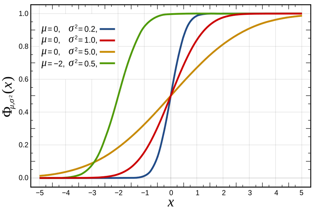
Mathematically, the normal distribution is defined by its probability density function (PDF). ^[6] This function describes the relative likelihood for a random variable to take on a given value. ^[6] The equation, which involves the constant $ee$ (Euler's number), $\pi \backslash pi$, $\mu \backslash mu$, and $\sigma \backslash sigma$, defines the exact shape of the bell curve. ^[6]

$$f(x)=\frac{1}{\sigma \sqrt{2\pi }}{e}^{-\frac{1}{2}{\left(\frac{x-\mu }{\sigma }\right)}^2}f(x)\; =\; \backslash frac\{1\}\{\backslash sigma\; \backslash sqrt\{2\backslash pi\}\}\; e^\{-\backslash frac\{1\}\{2\}\backslash left(\backslash frac\{x-\backslash mu\}\{\backslash sigma\}\backslash right)^2\}$$

While the equation itself looks complex, its role is simply to mathematically formalize the visual properties we observe: the peak at $\mu \backslash mu$, the control over spread by $\sigma \backslash sigma$, and the requirement that the total area under the curve must equal exactly 1, representing 100% probability. ^[3][6][9] The use of this function is what allows computers and statistical tables to precisely calculate probabilities associated with specific ranges of data under the curve. ^[3]

# Practical Application

Understanding the normal distribution moves beyond theory when considering quality control or risk assessment. In manufacturing, for example, ensuring that the diameter of machine-produced bolts is normally distributed around the target specification is critical. ^[4] If the distribution is too wide (high $\sigma \backslash sigma$), too many bolts will be unusable because they are too big or too small. If the distribution is centered incorrectly (wrong $\mu \backslash mu$), all the bolts might be too large, even if the variation is low.

The reliance on the assumption of normality is high across many statistical tests, such as t-tests and ANOVA. ^[4] If a researcher suspects their data is heavily non-normal, they often must transform the data or use non-parametric statistical methods instead, demonstrating that verifying the distribution shape is an essential first step in any serious analysis. ^[1] Recognizing the characteristics—the symmetry, the defined center, and the predictable spread—is what allows us to categorize a collection of measurements as truly "normal" and apply the powerful mathematical tools that rely on that specific definition. ^[4]