What defines computational complexity?

Computational complexity centers on classifying computational problems based on the resources required by the most efficient known algorithms to solve them. It is fundamentally concerned not with how fast a specific computer runs a specific program, but rather with the inherent difficulty embedded within the problem itself, independent of any particular machine implementation. This discipline is generally divided into two closely related areas: algorithmic complexity, which measures the cost of a specific algorithm, and computational complexity theory, which classifies problems based on their intrinsic difficulty.

The measurement process quantifies the resources needed as a function of the size of the input, often denoted by the variable $n$ . The two primary resources considered are time, representing the number of computational steps, and space, representing the amount of memory storage needed. While both are crucial, time complexity often receives the most immediate attention when assessing the practicality of an approach.

# Resource Metrics

When analyzing an algorithm, practitioners seek to describe how the resource requirements scale as the input size grows. This relationship is typically described using asymptotic notation, most famously Big O notation. Big O notation provides an upper bound on the growth rate, describing the worst-case scenario for the algorithm.

For example, an algorithm with $O (n)$ complexity is called linear, meaning the time required grows directly proportionally to the input size. An algorithm running in $O (n^{2})$ is quadratic, which scales much faster as $n$ increases. Understanding this scaling is more important than knowing the exact time in seconds because seconds are dependent on hardware speed, programming language, and compiler efficiency, none of which are relevant to the theoretical definition of complexity.

It is important to distinguish between the specific cost of one algorithm and the complexity of the problem itself. If you have a problem that requires at least $O(n \log n)$ steps just to read the input (like sorting an unsorted list), then no algorithm, no matter how clever, can solve it faster than $O(n \log n)$ in the worst case. Therefore, the complexity of the problem establishes a lower bound on the required resources.

# Formal Models

To discuss complexity in a rigorous, mathematical manner, complexity theory relies on idealized computational models. The most common model used as the standard for theoretical analysis is the Turing machine. A Turing machine is an abstract mathematical concept that defines exactly what it means for something to be computable and how resources are consumed during that computation.

The reliance on a formal model like the Turing machine is key to the definition of computational complexity theory. If complexity were measured purely by the speed of a specific Intel chip running Python, the results would not be universal or timeless; they would change with the next processor generation. By basing analysis on the Turing machine—a model abstract enough to capture the essence of computation without being tied to current hardware—the resulting complexity classification for a problem remains constant.

While the Turing machine is the theoretical gold standard, other models are sometimes used for specialized analyses. For instance, RAM models (Random Access Machine) or algebraic computation models might be employed when analyzing problems better suited to those structures, but the complexity results derived from them are generally expected to be polynomially equivalent to those derived from a Turing machine, thanks to the Church-Turing thesis.

What defines an emerging infectious disease?

# Problem Classification

The real goal of computational complexity theory is not just to analyze algorithms, but to categorize the problems themselves into classes based on their inherent resource demands. These classes group problems that can be solved using similar levels of resources.

The most famous classification involves decision problems: problems whose answer is strictly "yes" or "no".

# Primary Classes

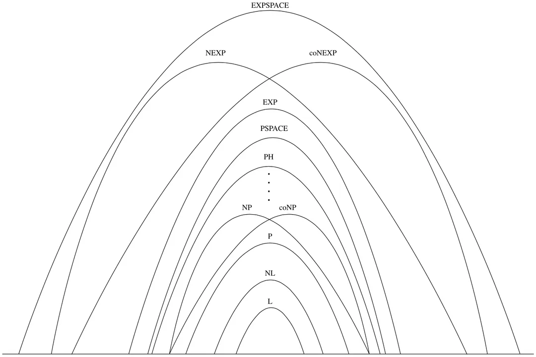
Two classes dominate the landscape of theoretical computer science: $\mathbf{P}$ and $\mathbf{NP}$ .

$\mathbf{P}$ (Polynomial Time) represents the set of decision problems that can be solved by a deterministic Turing machine in a time that is bounded by a polynomial function of the input size ( $O (n^{k})$ for some fixed $k$ ). Problems in P are generally considered tractable or efficiently solvable because the growth rate of the required time, even for very large inputs, remains manageable. Examples include sorting, finding the shortest path in a graph, or checking if two strings are identical.

$\mathbf{NP}$ (Nondeterministic Polynomial Time) is the set of decision problems where a yes answer can be verified quickly. Specifically, if someone gives you a potential solution (a "certificate"), a deterministic machine can check if that solution is correct in polynomial time. Crucially, NP does not mean "not polynomial"; it means "verifiable in polynomial time". Satisfiability (SAT) and the Traveling Salesperson Problem (when framed as a decision question—"Is there a tour shorter than $k$ ?") are classic examples of NP problems.

The relationship between these two classes forms the most significant open question in computer science: Is $\mathbf{P} = \mathbf{NP}$ ?. If $P = N P$ , it would mean that any problem whose solution can be quickly verified can also be quickly solved from scratch. If $P \neq NP$ , it implies that some problems are fundamentally harder to solve than they are to check.

# Beyond P and NP

The classification extends much further. Problems that are in NP but are strongly believed not to be in P are called NP-complete problems. These are the "hardest" problems in NP; if anyone found a polynomial-time solution for just one NP-complete problem, it would instantly imply that $P = N P$ .

Other key classes include $\mathbf{PSPACE}$ (problems solvable using polynomial space, regardless of time) and problems that are not even solvable by a Turing machine, known as undecidable problems. The existence of undecidable problems, like the Halting Problem, establishes the absolute limits of computation itself.

# Algorithmic Cost Versus Inherent Difficulty

While the theory classifies problems, working software engineers deal daily with algorithmic complexity, the cost of the code they write. A common point of confusion is treating the analysis of a single algorithm as synonymous with the theory of computational complexity. While related, they operate at different levels of abstraction.

Consider two different algorithms designed to sort a list of $n$ numbers. Algorithm A might be Merge Sort, running in $O(n \log n)$ . Algorithm B might be Bubble Sort, running in $O (n^{2})$ in the worst case. The problem of sorting has a known lower bound of $O(n \log n)$ on comparison-based models. Thus, Merge Sort is considered efficient because it matches this lower bound, while Bubble Sort is inefficient because it is slower, even though both are theoretically in $\mathbf{P}$ .

This difference is pragmatic. When an input size ( $n$ ) is small—say, $n<100$ —the $O (n^{2})$ Bubble Sort might actually run faster than Merge Sort due to lower constant factors, better cache locality, or simpler implementation overhead. However, as $n$ grows into the millions, the $O (n^{2})$ approach quickly becomes computationally infeasible, while the $O(n \log n)$ approach remains perfectly tractable.

To better reflect real-world constraints, complexity analysis sometimes moves beyond the strict worst-case boundary. Average-case complexity looks at the expected resource use across a random distribution of inputs, which can provide a more optimistic, yet sometimes misleading, picture than the guaranteed upper bound.

When selecting an approach for a new system, a programmer should always estimate the likely range of $n$ they will encounter. If you are dealing with inputs where $n$ will never exceed a few thousand, an $O (n^{3})$ solution might be acceptable if it's simpler to code and debug than a complex $O(n \log n)$ alternative. Conversely, if the input size is unpredictable and could potentially reach millions, one must ruthlessly optimize for the best possible asymptotic class, often sacrificing initial simplicity for long-term scalability. This consideration of input scale relative to asymptotic growth is a practical application of complexity theory.

How do quantum computers differ from classical ones?

# Nuances in Measurement

Defining complexity precisely requires careful management of what is being counted. In a simple Turing machine model, every transition step counts as one unit of time, and every cell written to on the tape counts as one unit of space. However, modern computing involves much richer instruction sets.

Consider arithmetic operations. In a basic model, adding two single-digit numbers takes one step. But what about adding two numbers that have $k$ digits? If the model assumes that arithmetic operations on arbitrarily large numbers take constant time, the analysis can become inaccurate for certain problems involving massive integers (like cryptography). For these specialized areas, complexity analysis must sometimes account for the number of bits required to represent the numbers, making the input size $n$ relate to the logarithm of the numerical value. This subtlety shows that even the definition of a "single step" depends on the context of the problem being studied.

Another nuance involves the distinction between deterministic and nondeterministic computation, which is central to the $\mathbf{P}$ versus $\mathbf{NP}$ gap. A deterministic machine follows one path of computation. A nondeterministic machine, in essence, can "guess" the correct path or explore all paths simultaneously. The fact that verification (NP) is easy while solving (P) might be hard suggests that nondeterminism offers a profound computational advantage that we currently lack in our physical machines.

# The Scope of Study

The field of computational complexity is broader than just time and space on a Turing machine; it encompasses various computational resources and different models of computation. Researchers investigate complexity relative to quantum computation models or parallel computation models, seeking to understand how resource utilization changes when multiple processors are available or when quantum effects are permitted.

Fundamentally, the study defines the boundaries of what is practically solvable versus what is theoretically solvable but practically impossible. Problems that require exponential time, $O (2^{n})$ , are considered intractable for large $n$ because the resource demands grow too quickly for even the world's largest supercomputers to handle within a meaningful timeframe. For instance, an input size of $n = 100$ might require $2^{100}$ steps, a number far exceeding the number of atoms in the observable universe.

Understanding these boundaries allows researchers to guide algorithm design efforts away from hopeless causes and toward approaches that promise efficiency. If a problem is proven to be NP-complete, an attempt to find a fast, general solution is unlikely to succeed; the effort is better spent looking for an approximate solution, restricting the input domain, or developing a heuristic that works well on average rather than in the worst case.

A simple mental checklist for developers analyzing a new algorithm involves first identifying $n$ (the variable input size), then mapping the major operations (loops, recursions) to their corresponding time costs, and finally simplifying the expression to its dominant term (the Big O). For example, if an algorithm involves reading an input of size $n$ and then iterating over all pairs within that input, the complexity is $O (n) + O (n^{2})$ , which simplifies to $O (n^{2})$ . If, however, the algorithm involves an outer loop that runs $n$ times, and inside that loop, it calls a subroutine known to be $O (2^{n})$ , the overall complexity is dominated by the exponential term, resulting in $O(n \cdot 2^n)$ , signaling a structure that must be avoided for scaling inputs. This hierarchy, from the theoretical Turing machine down to the practical scaling factors of a specific routine, provides the complete picture of what defines computational complexity..