How do algorithms scale with input size?

Understanding how an algorithm's performance shifts as the data it processes grows is fundamental to writing efficient software. This relationship, often framed around the input size, $N$ , determines whether a solution remains practical when faced with real-world data volumes or grinds to a halt when $N$ gets large. ^[1]^[2] Simply timing an algorithm on one set of data tells us very little about its future behavior; we need a mathematical language to describe this growth rate abstractly. ^[1]

# Scaling Language

The accepted way to quantify this scaling behavior is through Big O notation. ^[1]^[5] This mathematical tool provides an abstraction layer over the actual execution time measured in seconds, which can fluctuate based on the specific machine, compiler, or the current load on the system. ^[2] Big O notation focuses exclusively on the rate at which the number of operations grows as the input size $N$ approaches infinity. ^[1]^[5] It ignores constant factors and lower-order terms, concentrating only on the dominant term that dictates the upper bound of the growth curve. ^[1]^[5] For instance, an algorithm requiring $5 N^{2} + 100 N + 50$ operations is simplified to $O (N^{2})$ because for very large $N$ , the $N^{2}$ term overwhelms the others. ^[1]

# Growth Categories

Algorithms fall into distinct categories based on their Big O classification, which dictates how quickly their time requirement increases relative to $N$ . ^[2]^[6]

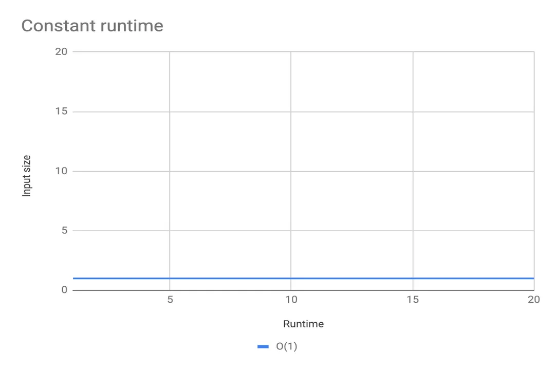
# Constant Time

The most desirable scaling is constant time, denoted as $O (1)$ . ^[2]^[6] In this scenario, the time taken to execute the algorithm is entirely independent of the input size $N$ . ^[2] Retrieving an element from an array by its index or looking up a key in a well-implemented hash map are classic examples. ^[6] No matter if you have ten items or ten million, the number of steps remains fixed. ^[2]

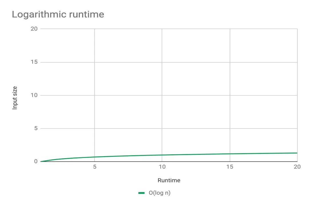
# Logarithmic Growth

Next is logarithmic time, or $O(\log N)$ . ^[2]^[6] This performance is exceptionally good for large datasets. The time required increases slowly, as the input size is effectively halved or divided by a constant factor in each step. ^[2] Binary search is the archetypal example of this efficiency. ^[2]^[6] If the input size doubles, the time taken increases by only one constant step, making it highly scalable. ^[6]

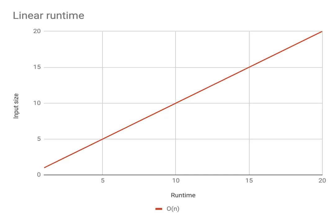
# Linear Scaling

When an algorithm takes time directly proportional to the input size, it is linear time, $O (N)$ . ^[2]^[6] If you double the input, you double the execution time. ^[2] Simple operations like iterating through an entire list once (a single for loop over the input) fall into this category. ^[6] This is generally considered very good performance, often the best achievable if every piece of input must be examined at least once. ^[2]

# Quasilinear Performance

The next tier, $O(N \log N)$ , is often seen in highly optimized sorting algorithms like Merge Sort or Heap Sort. ^[6] This performance is slightly worse than pure linear but significantly better than polynomial scaling. ^[6] Since $\log N$ grows so much slower than $N$ , this performance is often acceptable for very large inputs where simple $O (N)$ algorithms are too slow or $O (N^{2})$ is intractable. ^[1]

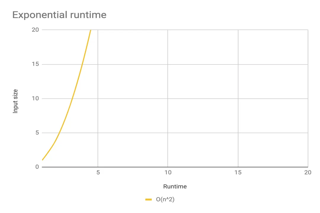
# Polynomial Growth

Algorithms that take quadratic time, $O (N^{2})$ , require time proportional to the square of the input size. ^[2]^[6] This usually occurs when nested loops process the entire input set against itself, such as in a basic Bubble Sort or Selection Sort implementation. ^[6] Doubling the input size quadruples the required time. For inputs in the tens of thousands, this rapidly becomes unworkable. ^[2] Even worse are cubic ( $O (N^{3})$ ) or higher polynomial complexities, which are generally only practical for tiny inputs. ^[6]

Complexity	Notation	Scaling Description	Typical Example
Constant	$O (1)$	Time does not change with $N$	Array index access
Logarithmic	$O(\log N)$	Time grows very slowly	Binary Search
Linear	$O (N)$	Time grows directly with $N$	Single list traversal
Quasilinear	$O(N \log N)$	Better than polynomial	Merge Sort
Quadratic	$O (N^{2})$	Time grows by the square of $N$	Simple nested loops

What distinguishes deterministic from probabilistic algorithms?

# Measuring Time vs. Value

A crucial distinction when assessing scaling is recognizing the difference between the size of the input and the magnitude of the values within the input. ^[4] Big O notation primarily measures the time complexity in terms of the number of items, $N$ . ^[4]^[7] Consider two scenarios for sorting a list of numbers. In the first, $N = 1000$ numbers are small integers (e.g., 1 to 100). In the second, $N = 1000$ numbers are extremely large, perhaps 500-digit numbers. ^[4] An algorithm like Quick Sort, which is $O(N \log N)$ in terms of item count, will take significantly longer to compare two 500-digit numbers than two small integers, even though the $N$ (the count of items) is the same. ^[4] The time taken for comparisons or arithmetic operations on large data types contributes to the constant factor hidden within the Big O classification, but the asymptotic scaling is still determined by $N$ . ^[4] The input size $N$ dictates the number of steps, while the data magnitude influences how long each step takes. ^[4]

# Surprising Growth Curves

While the general trend is that performance degrades as $N$ increases, this isn't universally true across all possible performance metrics or input distributions. ^[3]^[5] It is mathematically possible for an algorithm's runtime to decrease as the input size increases, though these situations are often highly specific or depend on how the complexity is measured. ^[3]^[5]

One common area where this seeming paradox arises is when comparing the average-case complexity versus the worst-case complexity. ^[3] For instance, Quick Sort is notoriously $O (N^{2})$ in its worst-case scenario—when the pivot selection consistently results in highly unbalanced partitions—but its average-case complexity is the much better $O(N \log N)$ . ^[3] If an input distribution guarantees that the worst-case pivot scenarios never happen, the algorithm might appear to scale better than its worst-case notation suggests. ^[3] Similarly, algorithms designed for highly specific data structures or data states might exhibit surprising behavior. If an algorithm's initialization or setup time is extremely high, but subsequent operations become exceptionally fast for larger subsequent inputs, the overall observed time might seem to decrease as the initial N grows, especially if the definition of "input size" is being shifted across multiple runs. ^[3] This often involves algorithms that have a heavy, non-scalable setup cost followed by a highly efficient scaling component. ^[5]

When developing an algorithm, it is vital to remember that the Big O classification describes the behavior as $N$ tends towards infinity. For small, real-world data sets, the actual wall-clock time is heavily influenced by the constant factors hidden by the notation. ^[1] An $O (N^{2})$ algorithm with a very small constant factor—perhaps performing only a few simple memory accesses per iteration—might outperform a highly complex, but theoretically superior, $O(N \log N)$ algorithm until $N$ reaches a specific crossover point. ^[1] If the operational environment ensures that $N$ will never pass this crossover threshold, selecting the simpler, constant-heavy algorithm can be the more pragmatic choice, prioritizing ease of coding and debugging over asymptotic perfection. ^[1]

What limits population size in nature?

# Analyzing Practical Constraints

When designing systems, recognizing the scaling behavior allows engineers to set practical limits on data handling. ^[9] If a service relies on a proprietary matching algorithm that is $O (N^{3})$ , expecting it to handle more than a few hundred inputs reliably is unrealistic. ^[6] Conversely, if a recommendation engine runs in $O(\log N)$ , it can handle millions of users with minimal performance degradation, offering a much safer long-term bet. ^[2] The primary goal is often to select an algorithm whose growth rate is manageable for the largest expected input size, not just the current size. ^[9]

Engineers must consider the total computational cost, which is a combination of the growth rate and the constant overhead. ^[1] For large-scale production systems, the asymptotic behavior—the Big O—is the ultimate constraint, forcing architects to move away from $O (N^{2})$ and worse as data grows. ^[2] However, for smaller, localized tasks where the input size is bounded and relatively small (say, under 10,000 elements), simplicity and low constant factors often win out over asymptotic elegance. ^[1] Understanding scaling is thus not just an academic exercise but a critical factor in architectural decision-making, balancing theoretical efficiency with real-world implementation constraints and predictable performance ceilings. ^[9]