What limits measurement precision?

The effort to measure something accurately is often met with barriers, some stemming from the tools we use, others from the laws of nature itself. Understanding what curtails our ability to achieve perfect measurements requires distinguishing between the concepts of accuracy and precision first, as they are frequently confused in casual conversation.

In simple terms, accuracy refers to how close a measurement is to the true or accepted value of what is being measured. If you aim for a target and consistently hit the bullseye, your aiming is accurate. Conversely, precision describes how close repeated measurements are to each other, regardless of whether they are near the true value. High precision means low random error; you might be consistently hitting the same spot on the target, but if that spot is far from the center, your measurements are precise but not accurate. A measurement reported as $10.00 \pm 0.02 \text{ cm}$ conveys both an estimate of the value and its associated uncertainty, which is key to understanding limitations.

# Terminology Explained

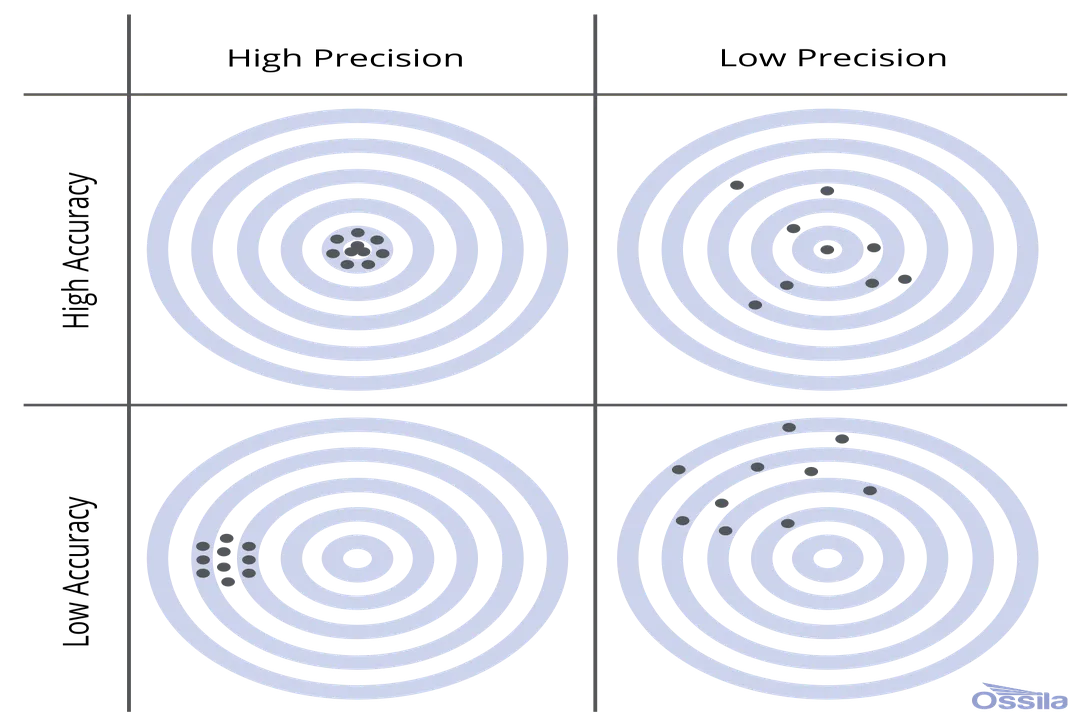
Distinguishing between these two concepts is critical for interpreting any experimental result. Imagine a set of darts thrown at a board. If all the darts land in a tight cluster far from the center, they demonstrate high precision but low accuracy. If the darts are scattered widely around the board but their average position is near the center, the result shows high accuracy but low precision. Ideally, a measurement technique strives for both high accuracy and high precision, meaning the readings cluster tightly around the true value.

The limitations on these qualities are rooted in different sources. The gap between the measured value and the true value is often addressed by concepts like uncertainty and tolerance. Uncertainty reflects the doubt about the result of any measurement, expressed as a range. Tolerance, particularly in engineering contexts, defines the acceptable variation allowed for a component or process to still be considered functional. While precision relates to the scatter of random measurements, uncertainty attempts to quantify the overall expected error, encompassing both systematic and random sources.

# Error Sources

Measurement limitations are broadly categorized by the nature of the error introduced. Errors can generally be classified as either systematic or random, and each impacts accuracy and precision differently.

# Systematic Errors

Systematic errors, often called determinate errors, consistently shift measurements in the same direction—either too high or too low. These errors prevent a measurement from being truly accurate, even if the readings are tightly clustered (i.e., high precision). Think of a digital scale that always reads 0.5 grams heavy; every reading will be systematically off by that amount.

Potential causes for systematic errors are numerous. They can stem from poorly calibrated instruments, where the zero point is incorrect or the scale factor is wrong. In chemistry, for example, using impure reagents or having a thermometer that consistently reads two degrees too high introduces systematic error. These types of errors are generally correctable once identified, often through comparison with a known standard—a process called calibration.

# Random Errors

Random errors, conversely, are indeterminate errors that cause measurements to fluctuate unpredictably around the true value. This type of error directly limits precision because successive readings will not agree with one another. The scatter in the results is the manifestation of random error.

Sources of random error include small, uncontrollable fluctuations in the environment—like slight variations in temperature or air currents—or the inherent limitations in observing or reading an analog scale. For instance, a human operator estimating between the lines on a ruler will introduce a small, random uncertainty in every reading they take. Unlike systematic errors, random errors cannot be entirely eliminated, but their effect on the final reported result can be minimized by taking many measurements and calculating the average.

What limits data transmission speed?

# Instrument Capability

The physical makeup and design of the measuring device itself impose hard limits on precision and accuracy. No matter how careful the user, a tool can only resolve down to a certain level.

# Resolution Limits

The resolution of an instrument is the smallest increment it can detect or display. A ruler marked only in centimeters has a resolution limit of 1 cm. If you use that ruler to measure a pencil that is $14.3$ cm long, you are forced to estimate the decimal place, introducing uncertainty. A more precise instrument, like one marked in millimeters, offers a resolution of $0.1 \text{ cm}$ , allowing for a more accurate estimate of the $14.3 \text{ cm}$ length.

In optics, for example, the resolution of a microscope or camera system is fundamentally limited by the wavelength of light used for illumination and the numerical aperture of the objective lens. This is a physical constraint dictated by the nature of light itself. Similarly, electronic sensors have internal noise levels that establish a minimum detectable signal, setting an inherent floor on their precision.

# Environmental Drift

A subtle but powerful limitation arises from environmental factors interacting with the measuring instrument over time. Temperature changes can cause materials to expand or contract, altering the physical length of a measuring stick or the internal components of an electronic sensor. If a standard weight used for calibration has a known mass at $20^\circ \text{C}$ , but the room temperature is $25^\circ \text{C}$ during the actual measurement, this temperature difference introduces a systematic error unless the instrument or standard is corrected for thermal expansion or contraction. This environmental drift can slowly degrade both accuracy and precision if the instrument is not frequently re-verified against a known standard under controlled conditions.

If we consider measurement as an inventory check, a systematic error is like having a known accounting discrepancy—say, a missing $100$ in the till every day. We can fix that with a correction factor. A random error, however, is like having unpredictable petty cash transactions every hour; we can only estimate the net effect by looking at a large ledger of transactions over a month.

# Operator Influence

Even with a perfect, zero-error instrument, the human element introduces limitations. Reading an instrument requires interpretation, which is susceptible to human variation.

# Parallax Error

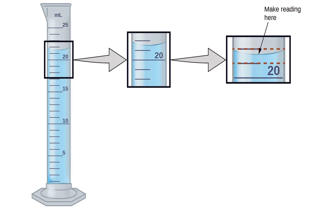
A classic example of human error limiting accuracy is parallax error. This occurs when the observer's eye is not positioned directly perpendicular to the scale being read, causing the apparent position of the measurement mark to shift relative to the object being measured. For instance, reading the meniscus of a liquid in a graduated cylinder from above or below the horizontal line will result in a consistently inaccurate reading in one direction or the other, creating a systematic error specific to that observer's technique.

# Reading Estimation

As mentioned with resolution, estimation is required when the measurement falls between the finest divisions on the scale. Standard practice in many fields dictates that the final recorded digit should be an estimation, typically one decimal place beyond the finest graduation on the instrument. For example, if the finest markings are $0.1$ units apart, the reading should be reported to the $0.01$ unit place. The precision of the result is thus capped by the visual acuity and judgment of the person taking the reading.

What limits human lifespan biologically?

# Physical Constraints

Beyond the practical limits of tools and human perception, there exist fundamental, inescapable limitations imposed by the laws of physics governing the universe.

# Quantum Limits

At the most fundamental level, the precision of any measurement is constrained by quantum mechanics, specifically the Heisenberg Uncertainty Principle. This principle dictates that certain pairs of complementary variables, such as a particle's position and momentum, cannot both be known with arbitrary precision simultaneously.

The relationship is expressed mathematically as $\Delta x \Delta p \ge \hbar/2$ , where $\Delta x$ is the uncertainty in position, $\Delta p$ is the uncertainty in momentum, and $\hbar$ (h-bar) is the reduced Planck constant. To measure a particle's position ( $\Delta x$ ) with extreme accuracy (making $\Delta x$ very small), the uncertainty in its momentum ( $\Delta p$ ) must necessarily become very large. Conversely, trying to pin down an object's momentum too precisely blurs our knowledge of where it actually is. This is not a limitation of our technology; it is a fundamental property of reality.

This principle applies to energy and time as well ( $\Delta E \Delta t \ge \hbar/2$ ). If you try to measure the energy of a quantum state over a very short time interval ( $\Delta t$ is small), the resulting energy measurement ( $\Delta E$ ) will have a correspondingly large uncertainty. This effectively sets an absolute limit on measurement precision in physics that no amount of better engineering can overcome.

# Zero Point Energy

Another quantum mechanical consideration involves zero-point energy. Even in the absolute ground state of a system, there is residual energy present, meaning no system is ever perfectly static or at absolute zero energy, which introduces inherent noise or jitter into the system that can affect highly sensitive measurements.

# Reporting Results

How we communicate the limitations of our measurements is as important as the measurement itself. The way results are recorded directly reflects the measurement precision achieved.

# Significant Figures

The concept of significant figures provides a method for recording data that communicates the precision inherent in the measurement process. Every non-zero digit in a measurement is considered significant, as are interior zeros. Trailing zeros are significant only if the measurement includes a decimal point (e.g., $5.00 \text{ g}$ has three significant figures, while $500 \text{ g}$ might only have one).

The rules for combining measurements, such as addition/subtraction (limited by the least precise decimal place) and multiplication/division (limited by the fewest number of significant figures), ensure that the calculated result does not claim more precision than the least precise component measurement allowed. If you measure a length as $12.4 \text{ cm}$ (three significant figures) and multiply it by a constant known exactly (infinite precision), the result must still only be reported with three significant figures to reflect the initial measurement's limitation.

# Tolerance and Uncertainty Reporting

In metrology (the science of measurement), quantifying the uncertainty associated with a value often involves more sophisticated reporting than just significant figures, especially when dealing with tolerances. When specifying a part with a nominal dimension of $5.00 \text{ mm}$ with a tolerance of $\pm 0.05 \text{ mm}$ , the acceptable range is $4.95 \text{ mm}$ to $5.05 \text{ mm}$ .

When generating an uncertainty value, $\pm U$ , where $U$ is the expanded uncertainty, scientists often use a coverage factor, such as $k = 2$ , which corresponds to a $95$ confidence level that the true value lies within the reported range. This acknowledges that while random errors suggest a high probability of being near the average, there remains a small chance, particularly due to unknown systematic effects or low-frequency noise, that the true value lies slightly outside the narrowly defined precision range derived only from standard deviation.

The overall limiting factor in a complex measurement chain is always the component that contributes the largest relative uncertainty. If a highly precise sensor ( $0.01$ uncertainty) is used with a sample preparation step that introduces a $1$ contamination error, the overall measurement precision will be limited by the $1$ contamination, making the excellent sensor performance nearly irrelevant to the final accuracy. This points to an actionable takeaway: always analyze the entire measurement process, not just the final instrument, to identify the true bottleneck limiting precision. The focus must shift from minimizing random noise in the best component to controlling the largest source of systematic or procedural deviation.