How does variance measure spread?
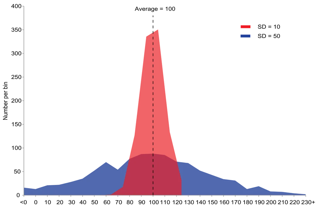
Variance provides a precise mathematical answer to a fundamental question in data analysis: How spread out are the data points from the center of the distribution? While we often look at the average, or the mean, to understand where the data clusters, the average alone tells us nothing about the consistency or variability within that data set. [2][5] Understanding variance means understanding dispersion—how much deviation exists between individual observations and that calculated central point. [3][7]
Think of two groups of students taking the same exam. Both groups might have an average score of 75%. Group A consists of students who scored between 72% and 78%. Group B has students who scored anywhere from 40% to 100%. Both have the same mean, but the spread is vastly different. Variance quantifies this difference, giving us a single number to represent the chaos, or lack thereof, in the scores. [2]
# Spread Definition
Dispersion, or spread, is a key component of descriptive statistics, alongside measures of central tendency. [5] Range is the simplest measure of spread—it is just the difference between the highest and lowest values in a set. [3][4] However, range is extremely susceptible to outliers; one unusually high or low score can drastically change the range without reflecting the typical behavior of the majority of the data points. [3] Variance offers a more sophisticated and stable look at this dispersion because it considers every data point in its calculation. [1][6] It measures the average squared distance of each observation from the mean. [1][5]
# Calculation Mechanics
The process for calculating variance involves several distinct steps, which build upon each other to capture the total deviation across the entire data set. [2]
First, you must establish the center point by calculating the mean ( or ) of the data set. [1]
Next, for every single data point () in your set, you find its deviation from the mean (): . [1][2]
This deviation step is where the core insight of variance emerges. If you simply summed up these deviations, the positive distances (points above the mean) would perfectly cancel out the negative distances (points below the mean), always resulting in zero. [1][5] This is why the next step is necessary: squaring each deviation . [1][2] Squaring serves two purposes: it eliminates the negative signs, and, more importantly for the metric itself, it disproportionately increases the penalty for values that are far from the mean. A data point twice as far from the mean contributes four times the squared deviation to the total sum compared to a point only half as far away. This inherent weighting means variance is keenly sensitive to large individual differences from the average. [5]
Once all squared deviations are calculated, you sum them up to get the sum of squares.
Finally, you calculate the average of those squared deviations to arrive at the variance ( for a population or for a sample). [1][5]
The distinction between population and sample variance centers on the denominator used in this final averaging step. [1][5] For an entire population, you divide the sum of squares by , the total number of observations. [1] When dealing with a sample drawn from a larger population, we divide by , where is the sample size. This adjustment, known as Bessel's correction, is used because using would typically underestimate the true variance of the larger population from which the sample was drawn. [1][5]

# Unit Dilemma
While the steps clearly describe how data spreads, the resulting value for variance itself is often difficult to interpret directly in a practical sense. [3] If you are measuring the spread of house prices in dollars, the variance will be expressed in squared dollars. If you are measuring the spread of heights in centimeters, the variance is in square centimeters. [2] This squared unit makes direct comparison to the original data challenging for non-statisticians.
For instance, knowing the variance of customer wait times is $144$ seconds squared doesn't immediately tell you, "On average, customers wait seconds too long." To make the measure intuitive and put it back onto the original scale of measurement, we take the square root of the variance. [2][3] This operation yields the standard deviation ( or ), which is the single most common way to express spread because it shares the same units as the original data and the mean. [2][3]
# Comparing Dispersion Metrics
Variance is a mathematical workhorse, but it exists alongside other measures of spread, each offering a different perspective on data distribution. [4]
| Metric | Calculation Basis | Interpretation | Key Feature |
|---|---|---|---|
| Range | Difference between Max and Min | Total observed spread | Extremely simple; highly sensitive to outliers. [3] |
| Variance () | Average of squared deviations from the mean | Average squared distance from the center | Mathematically convenient but in squared units. [1][5] |
| Standard Deviation () | Square root of Variance | Average typical distance from the mean | Intuitive units; the most commonly reported spread measure. [2][3] |
When assessing data spread, you are essentially weighing the utility of easy interpretation (Range/Standard Deviation) against mathematical consistency (Variance). [3] For initial data exploration, range offers a quick boundary check. For reporting findings to a general audience, standard deviation is usually preferred. [2] However, for building statistical models or performing certain hypothesis tests, variance is the preferred input. [6]
# Statistical Utility
The reason variance remains a core concept, even with the difficulty of its squared units, lies in its superior mathematical properties for advanced analysis. [6] When dealing with multiple independent random variables, the variance of their sum is simply the sum of their individual variances. This property, known as additivity, does not hold for standard deviation, nor for the range. [6] This makes variance incredibly useful for creating and testing models, particularly in areas like regression analysis where we are decomposing total variation into explained and unexplained components.
If you are modeling the relationship between advertising spend and sales, the total variance in sales can be broken down into the portion explained by advertising and the portion that remains unexplained (the error term). The ability to add up the variance components of different explanatory factors is a mathematical convenience that simplifies complex statistical proofs and model building. [6]
This reliance on the squared term means variance inherently focuses on the magnitude of the differences rather than just their direction. Consider a scenario where you are trying to assess the risk associated with two investment portfolios. Portfolio X has returns that fluctuate wildly, sometimes gaining 20% and sometimes losing 20%. Portfolio Y has returns that hover closely around zero, maybe swinging between +2% and -2%. Both portfolios have a mean return close to zero. In this case, Portfolio X will have a vastly larger variance than Portfolio Y because the squaring operation magnifies the effect of those extreme 20% swings far more than it magnifies the small swings of Portfolio Y. In finance, variance (or standard deviation derived from it) acts as a quantifiable proxy for risk precisely because it penalizes large deviations so severely. [5]
If you are ever trying to isolate how much of the total variability in a process is attributable to a specific factor—say, comparing the consistency of two different suppliers in delivering materials—calculating the variance between the supplier means and then using the pooled variance within the supplier groups becomes a standard procedure, a technique built entirely upon the mathematical foundation that variance provides. [6] It is this mathematical predictability, stemming from the squaring, that cements variance as the fundamental measure of spread, even when standard deviation does the heavy lifting in final reporting.
Related Questions
#Citations
Variance - Wikipedia
Measures of spread: range, variance & standard deviation (video)
Maths and Stats - Variance, Standard Deviation and Standard Error
Measures of Spread - Range, Variance, and Standard Deviation
3.2: Measures of Spread - Statistics LibreTexts
How does the variance measure the information about the data?
2.7 Measures of the Spread of the Data - OpenStax
4.5.3 Calculating the variance and standard deviation
2.2.5 - Measures of Spread | STAT 200 - Statistics Online