What distinguishes laminar from turbulent flow?
The distinction between laminar and turbulent flow is not merely an academic curiosity in fluid mechanics; it dictates everything from how accurately we measure gas flow in a semiconductor process to the efficiency of air passing over an aircraft wing. Understanding the characteristics of these two fundamental flow regimes—smooth and orderly versus chaotic and irregular—is critical for any engineer or scientist working with moving fluids. At a basic level, laminar flow suggests an organized motion where fluid particles travel in parallel layers, while turbulent flow involves particles moving erratically, crossing streamlines, and creating complex, swirling motions known as eddies.
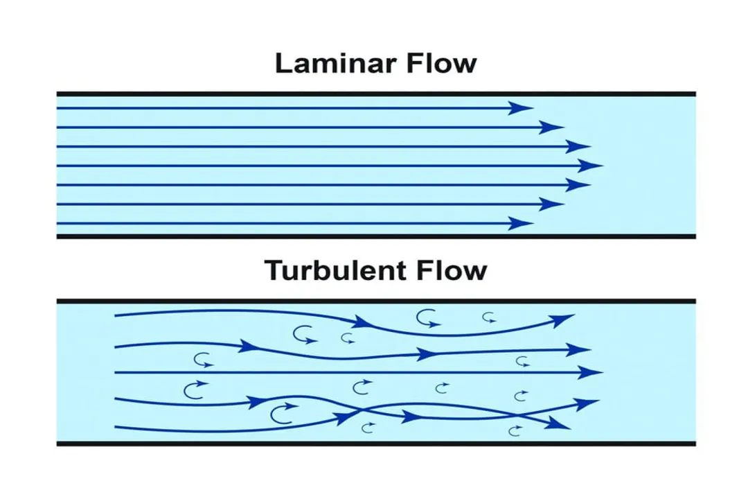
# Orderly Streamlines
Laminar flow represents the highly organized state of fluid movement. Imagine water moving slowly through a clean, straight pipe or a gentle stream meandering without obstacles; this visual captures the essence of laminar flow. In this condition, the fluid particles adhere to their respective paths, sliding smoothly over adjacent layers without intermixing. The velocity profile in a laminar condition is very predictable, often increasing monotonically from zero at the surface (due to the no-slip condition) to the full velocity in the center of the flow path. This orderly arrangement results in minimal energy loss within the fluid structure.
Laminar flow is typically observed when the fluid moves at relatively low velocities or when the fluid has high viscosity, meaning its internal resistance to flow is significant. Furthermore, maintaining laminar flow often requires an unobstructed path, free from sharp bends, valves, or other physical restrictions that could disrupt the parallel layers. In specific contexts, like the human circulatory system, laminar flow is a theoretical ideal—a good approximation for flow in medium and small blood vessels, though pulsatility often causes slight deviations, sometimes leading to a "plug flow" where velocities are nearly uniform across the lumen. Laminar flow characteristics can be further subdivided; for instance, water flow can be unidirectional (constant speed and direction), pulsatile (periodic speed fluctuations with constant direction), or oscillatory (constant speed but periodically changing direction).
# Chaotic Eddies
Turbulent flow stands in stark contrast, characterized by its noisy, unpredictable, and inherently chaotic nature. This regime arises when fluid velocities increase significantly or when the flow encounters a physical barrier, such as a rock in a river or a valve in a pipeline. When particles are forced to deviate from smooth paths, they collide, creating swirls, vortices, and eddies that cause mixing across the flow layers. This continuous, random fluctuation in both velocity magnitude and direction makes detailed, instantaneous prediction of turbulent flow extremely difficult.
The visible result of this chaos is often a highly mixed or aerated fluid; for example, the churning white appearance of whitewater rapids comes from air bubbles introduced by the turbulence. In an engineering sense, turbulence transfers kinetic energy from the large-scale organized motion (the macro scale) down to the smallest scale, eventually dissipating it as heat. While often seen as detrimental, this enhanced mixing capability is intentionally designed into processes like combustion, chemical manufacturing, and water treatment to speed up reactions. Conversely, in aerodynamics, turbulence within the boundary layer often increases drag on an object, making its mitigation a major focus for vehicle designers.

# Reynolds Number Predictive Tool
To move beyond simple observation and classify whether a flow is laminar, transitional, or turbulent, fluid dynamicists rely on a single, dimensionless quantity: the Reynolds number (). This number represents the ratio of inertial forces (the fluid's tendency to keep moving) to viscous forces (the fluid's internal resistance to deformation).
The calculation for the Reynolds number incorporates four key fluid and geometric properties:
Where:
- is the fluid density ().
- is the mean flow velocity ().
- is the characteristic dimension, like the pipe diameter ().
- is the dynamic viscosity ().
The interpretation of the resulting number guides the flow regime classification, although the exact cut-off values can vary slightly depending on the source or the specific geometry under study. Generally accepted ranges suggest:
- Laminar: is low, often cited as below $2000$ or $2300$.
- Turbulent: is high, often cited as above $3000$ or $3500$.
- Transitional: The range between the two—where the flow exhibits characteristics of both—is where things get interesting, commonly falling between $2300$ and $3500$.
It is important to note the variation in these cited thresholds. For instance, one source places the laminar threshold below $500$ and turbulence above $2000$ for streamflow analysis, while another suggests is laminar and is turbulent for pipe flow. This slight discrepancy underscores a key reality: the critical Reynolds number is not an absolute constant across all fields. Factors like the roughness of the pipe wall, the geometry of the conduit, and whether the fluid is blood or air mean that the flow may begin to transition at slightly different values than in idealized laboratory settings. For those working with heat exchangers, for example, the transitional zone between and $10,000$ is an area of uncertainty that designers actively try to avoid if possible, though the introduction of surface features like corrugations can influence the onset of turbulence within this range.
# Practical Impact and Design Goals
Whether a flow is laminar or turbulent has profound consequences for the performance of a system, meaning engineers sometimes strive for one while actively avoiding the other.
# Flow Meter Sensitivity
In the realm of flow measurement, precision is paramount, especially in high-value processes like pharmaceutical or chemical production. Many traditional thermal mass flow meters rely on the bypass principle and function optimally only when the inlet flow is perfectly laminar. If the flow arriving at the sensor is turbulent, the resulting chaotic movement introduces errors in measuring speed, pressure, and temperature, leading to inaccurate readings. Interestingly, flow meters based on the Coriolis principle, ultrasonic technology, or in-line Constant Temperature Anemometry (CTA) are generally unaffected by upstream turbulence, providing a clear distinction in instrumentation choice.
# Heat Transfer Efficiency
When the goal is to move heat rapidly—such as in a cooling system—turbulence is your friend. The mixing action of eddies dramatically increases the heat flux between a fluid and a surface. In contrast, laminar flow relies solely on less efficient conduction across the boundary layer, resulting in high heat transfer resistance. For engineers designing high-efficiency heat exchangers, operating in the high turbulent regime is generally the most efficient design point.
# Aerodynamics and Drag
For objects moving through a fluid, like an aircraft or a car, the interaction at the surface boundary layer is key to drag reduction. Generally, the goal is to maintain laminar flow along surfaces for as long as possible to minimize skin friction drag. However, this is one area where controlled turbulence is actively sought. Consider a golf ball: its dimples are intentionally placed to disrupt the laminar boundary layer, inducing a turbulent boundary layer further back on the ball. This induced turbulence causes the flow to remain attached longer to the surface, which surprisingly decreases the overall pressure drag, allowing the ball to travel farther. This demonstrates that the desired flow regime is entirely dependent on the specific engineering objective.

# Managing the Flow Environment
Since the ideal flow regime depends on the application—laminar for precise measurement and sterile environments, turbulent for aggressive mixing—controlling the flow transition is a core engineering task.
For applications sensitive to turbulence, like those using bypass thermal mass flow meters, several steps can be taken to restore order:
- Optimize Geometry: Eliminate unnecessary flow restrictions, such as adapters, valves, or tight elbows, as close to the sensor as possible.
- Ensure Straight Runs: Allow sufficient distance for the flow to naturally develop its profile. A common guideline suggests a minimum pipe length of ten times the pipe diameter immediately upstream of the instrument and four times the diameter downstream. This length helps shepherd the flow from a disturbed state into a more organized profile.
- Apply Filters: If restrictions cannot be avoided, turbulence filters or flow conditioners can be installed to actively smooth the flow before it reaches sensitive equipment.
# Computational Modeling Nuances
When designers cannot test physically, they turn to Computational Fluid Dynamics (CFD) tools to predict flow behavior. Modeling purely laminar flow is relatively simple, as the governing Navier-Stokes equations can be solved directly with good accuracy.
Turbulence presents a computational hurdle. To directly simulate every swirling eddy in a turbulent flow (Direct Numerical Simulation, or DNS) is often computationally prohibitive because the required resolution scales with the Reynolds number cubed. Therefore, engineers resort to statistical approximations. The most common methods are Reynolds-averaged Navier-Stokes (RANS) models, such as the Spalart-Almaras (SA) or two-equation models like k- SST. These models provide time-averaged results based on empirical data. A more advanced, but more costly, approach is Scale-Resolving Simulation (SRS), like Large Eddy Simulation (LES), which solves for the larger eddies explicitly while modeling the smaller ones, offering a time-dependent view of the flow structure.
When simulating complex industrial geometries, the greatest care must be taken in the transitional zone. Assuming a flow is fully turbulent when it is actually in transition (e.g., around $2500$) can cause a CFD model to over-predict the shear stress on the walls, leading to inaccurate predictions of wall interaction. This is why sophisticated CFD packages incorporate specialized transition modeling concepts, like Local-Correlation-based Transition Modeling (LCTM), to accurately capture the point where smooth layers begin to break down.
# Flow in Medical Imaging
The concepts of flow regimes are also relevant outside of traditional pipe and aerospace engineering, specifically within the context of Magnetic Resonance Imaging (MRI). When imaging blood flow, the flow pattern dictates the resulting MR signal, which is vital for techniques like MR angiography.
In blood vessels, the flow is generally considered laminar, characterized by predictable velocity layers. However, this flow pattern is often blunted away from the theoretical parabolic profile due to the pulsatile nature of the heart's pumping action. When velocities exceed a critical threshold or when the vessel geometry changes sharply—such as at bifurcations or past a narrowing called stenosis—the flow becomes turbulent, exhibiting random velocity fluctuations.
A related, but distinct, phenomenon seen in MRI is vortex flow. While turbulence involves rapid, random fluctuations, vortex flow describes localized, slower swirling or countercurrent motion that has separated from the main flow streamlines, often seen in aneurysms. Both turbulent flow and vortex flow complicate the acquisition and interpretation of MR angiography images because they distort the expected signal patterns.
| Feature | Laminar Flow | Turbulent Flow |
|---|---|---|
| Particle Movement | Smooth, parallel layers, orderly | Chaotic, random, non-linear |
| Velocity | Low and relatively constant | High and fluctuating between layers |
| Mixing/Interaction | Minimal particle mixing between layers | Significant mixing and formation of eddies/swirls |
| Dominant Force Ratio | Viscous forces dominate over inertial forces | Inertial forces dominate over viscous forces |
| Desirable For | Accurate flow measurement, sterile ventilation | Heat transfer maximization, fluid mixing |
| Example | Slow, straight stream; water tubing | Whitewater rapids; flow past a sharp bend |
Ultimately, the difference between laminar and turbulent flow boils down to the relationship between inertial drive and viscous damping, quantified by the Reynolds number. Mastering this relationship allows engineers to intentionally design systems that exploit the efficiency of orderly flow or harness the power of chaotic mixing.
Related Questions
#Citations
The Differences Between Laminar vs. Turbulent Flow
Laminar vs. Turbulent Flow: Difference, Examples, and ...
Laminar or Turbulent Flow
Laminar vs. Turbulent Flow | Definitions, Differences & ...
Comparison of Laminar and Turbulent Flow
Laminar v turbulent
can someone please describe and define laminar and ...
Understanding laminar vs turbulent flow in measurements