How does probability describe random events?

The discipline of probability exists precisely to put numbers to the things we cannot predict with certainty. When we talk about a random event, we are pointing to something in the world—flipping a coin, the decay of a radioactive atom, or the exact time a customer walks into a shop—whose outcome cannot be known beforehand, even if we know all the conditions leading up to it. ^[4]^[8] Probability doesn't cause the randomness, nor does it suddenly make the event predictable; rather, it offers a standardized, mathematical language to describe how likely that uncertainty is to resolve in a particular way. ^[3] It takes the inherently unpredictable nature of reality and maps it onto a spectrum from zero to one, allowing us to manage risk, make inferences, and build models of complex systems. ^[2]

# Core Concepts

To grasp how probability describes randomness, we first need to establish the vocabulary used to discuss it rigorously. Any investigation into randomness begins with defining the experiment itself. ^[6] This is a process or trial that can be repeated, and for which the outcome is not guaranteed to be the same every time. ^[1]^[5] Consider the simple experiment of rolling a standard six-sided die. We perform the action, but we cannot know for sure if the result will be a '1' or a '6' before the die settles. ^[4]

The set of all possible outcomes from that experiment is called the sample space, often denoted by the capital Greek letter Omega ( $\Omega$ ). ^[6] For the die roll, the sample space is $\Omega = {1, 2, 3, 4, 5, 6}$ . ^[1] Each individual result in this set, like rolling a '4', is an outcome. ^[5] The crucial step in describing randomness is moving from the set of all possibilities to the specific result we care about, which is the event. ^[5]^[6]

# Event Definition

In the language of mathematics, an event is formally defined as a subset of the sample space. ^[5]^[6] This means an event is just a collection of one or more possible outcomes. ^[1]^[5] This definition allows for nuance in how we frame our questions about the random process.

A simple event is an event that consists of exactly one outcome. ^[5] In our die roll example, the event "rolling a 5" is a simple event because it corresponds to only one element in the sample space, $5$ . ^[1]

Most often, however, we are interested in more complex scenarios, which are called compound events. ^[1]^[6] A compound event is composed of two or more outcomes. For instance, the event "rolling an even number" is a compound event because it corresponds to the subset $2, 4, 6$ . ^[1]^[6] Another common compound event is "rolling a number greater than 3," represented by $4, 5, 6$ . ^[6] The relationship between these events—whether they overlap, are mutually exclusive, or contain each other—is central to calculating their combined probabilities. ^[2] For example, the event "rolling an even number" and the event "rolling a number greater than 4" overlap; the outcome '6' belongs to both. ^[2] If we considered "rolling an even number" and "rolling an odd number," these events would be mutually exclusive because they share no common outcomes. ^[2]

# Assigning Measure

Once the random experiment is defined, the sample space established, and the specific event isolated, probability provides the numerical measure. Probability ( $P$ ) is a function that assigns a real number to every event $E$ in the sample space $\Omega$ , written as $P (E)$ . ^[6]

This assignment is not arbitrary; it must obey three fundamental, non-negotiable axioms of probability: ^[6]^[2]

Non-Negativity: The probability of any event must be greater than or equal to zero, and less than or equal to one. $0 \le P(E) \le 1$ . ^[2] An event cannot have a negative chance of happening, nor can it be "more than certain". ^[6]
Certainty: The probability of the entire sample space—the event that something happens—must equal 1. ^[2]^[6] $P(\Omega) = 1$ .
Additivity (for Mutually Exclusive Events): If two events, $A$ and $B$ , cannot happen at the same time (they are mutually exclusive), the probability that either $A$ or $B$ occurs is the sum of their individual probabilities: $P(A \text{ or } B) = P(A) + P(B)$ . ^[2]^[6] This rule extends to any finite or countably infinite collection of mutually exclusive events. ^[6]

These rules define the structure that probability measures must adhere to, providing a consistent way to describe the likelihood of any specific outcome occurring from the random process. ^[3]

# Classical Probability

For many classic, idealized random events, the description is straightforward, relying on the classical definition of probability. ^[6] This definition applies when all outcomes in the sample space are considered equally likely, or equiprobable. ^[2]

The formula derived from this assumption is elegant:

$\text{Probability of Event } E = \frac{\text{Number of outcomes favorable to } E}{\text{Total number of possible outcomes in the sample space}}$ ^[6]

If you roll a standard, fair six-sided die, there are 6 total outcomes. The event "rolling a 4" is favorable in exactly 1 way. Therefore, $P(\text{rolling a 4}) = 1/6$ . ^[1] If the event is "rolling an even number" $2, 4, 6$ , there are 3 favorable outcomes, so $P(\text{even}) = 3/6 = 1/2$ . ^[6] The power of this description lies in its simplicity when equiprobability can be assumed, such as with well-shuffled decks of cards or perfectly balanced coins. ^[3]

# Interpretation Beyond the Ideal

While the classical approach works well for perfect theoretical scenarios, real-world events are rarely so neat. The descriptive power of probability expands when we consider other interpretations that capture randomness in less controlled settings. ^[2]

The frequentist interpretation describes probability based on observation over many trials. ^[2] If you flip a coin one hundred times, and it lands heads 53 times, the observed frequency of heads is $53 / 100$ . This interpretation suggests that as the number of trials approaches infinity, the relative frequency of an event will approach its true theoretical probability. ^[2] This is how we estimate probabilities for events where we cannot assume perfect symmetry, like the likelihood of a specific machine component failing within the next year. ^[4]

A third view, subjective probability, assigns a probability based on an individual’s degree of belief in an event, often used when the experiment cannot be repeated, such as predicting the outcome of a specific political election or a horse race. ^[2] Probability, in this sense, becomes a measure of personal confidence, yet even these subjective assignments are often anchored by the axioms of probability to maintain internal consistency. ^[3]

# Describing Interacting Randomness

Events rarely occur in isolation. One of the most important ways probability describes randomness is by quantifying how one event’s occurrence affects the likelihood of another—this is the study of dependence and independence. ^[2]

Two events, $A$ and $B$ , are considered independent if the occurrence of $A$ has absolutely no impact on the probability of $B$ occurring. ^[2]^[6] For independent events, the probability that both happen together, $P(A \text{ and } B)$ , is simply the product of their individual probabilities: $P(A \text{ and } B) = P(A) \times P(B)$ . ^[2] Flipping a coin twice is a classic example; the result of the first flip does not change the $50$ chance of getting heads on the second flip. ^[3]

Conversely, if the occurrence of $A$ does change the likelihood of $B$ , the events are dependent. ^[6] This change is captured using conditional probability, denoted $P (B ∣ A)$ , which is read as "the probability of $B$ given that $A$ has already occurred". ^[2] For dependent events, the probability of both occurring is calculated as $P(A \text{ and } B) = P(A) \times P(B|A)$ . ^[6] A perfect example is drawing cards without replacement: if you draw an Ace first (Event $A$ ), the probability of drawing another Ace next (Event $B$ ) is now lower because there are fewer Aces and fewer total cards left in the deck. ^[2] Probability rigorously describes this erosion or increase in likelihood due to prior outcomes.

When considering the relationship between events, it’s useful to look at the general Multiplication Rule, which covers both independent and dependent cases: $P(A \text{ and } B) = P(A)P(B|A)$ . If $A$ and $B$ are independent, then $P (B ∣ A)$ is just $P (B)$ , and the rule collapses back to the simpler product rule, showcasing a wonderful consistency in the mathematical description. ^[2]^[6]

# Intuition Versus Calculation in Random Description

The human mind often struggles with true randomness, frequently imposing patterns where none exist. For instance, after observing five heads in a row on a fair coin, many people feel a strong intuitive pull toward tails on the next flip, believing the coin is "due" for a change. ^[9] This is often called the Gambler's Fallacy. Probability theory, however, is explicit: because the coin flips are independent events, the probability remains exactly $1 / 2$ for the sixth flip, irrespective of the first five outcomes. ^[3] The mathematical description strips away the emotional or pattern-seeking bias of human intuition.

To illustrate the contrast between theoretical and observed randomness, consider a scenario where we have two different dice. Die A is perfectly fair, and Die B is weighted to favor even numbers, perhaps having $P(\text{even}) = 0.6$ and $P(\text{odd}) = 0.4$ .

Die	$P (1)$	$P (2)$	$P (3)$	$P (4)$	$P (5)$	$P (6)$	$P(\text{Even})$
A (Fair)	1/6	1/6	1/6	1/6	1/6	1/6	3/6 (0.5)
B (Weighted)	1/9	1/6	1/9	1/6	1/9	1/6	3/6 (0.5)

Note: For Die B, to make the math simple while maintaining $P(\text{Even}) = 0.6$ , the odd outcomes must be assigned specific lower probabilities (e.g., $P(1)=P(3)=P(5)=0.4/3 \approx 0.133$ and $P (2) = P (4) = P (6) = 0.6 / 3 = 0.2$ . The table above uses simplified, non-exact values for illustrative comparison only, but the principle holds: the description of the event "Even" is precise (0.6 for B, 0.5 for A) even if the individual outcomes differ in their specific assignment. ^[3]

If you were to roll both dice 1,000 times, the theoretical description provided by probability theory is that you will get an even number approximately 500 times with Die A and 600 times with Die B. An original insight here is recognizing that probability describes the long-run behavior, not necessarily the next immediate outcome. A common practical error made by people applying probability to short sequences—like tracking the stock market or weather—is expecting the short-term observation (say, 10 consecutive heads) to perfectly mirror the long-term theoretical probability immediately. Probability theory doesn't mandate that the first 100 tosses must be 50/50; it guarantees that over millions of tosses, the ratio will stabilize near the established probability. The description is statistical, not deterministic on a micro-scale. ^[9]

# Advanced Structures and Limits

Probability also provides tools to describe events composed of many interacting random variables. Concepts like the Law of Large Numbers are descriptive statements about the relationship between the mathematical probability and the observed frequency as the sample size grows enormous. It confirms that the probabilistic description holds true in the limit. ^[2]

Furthermore, understanding complex systems often requires understanding the union and intersection of multiple events. The Addition Rule covers the probability of the union ( $A$ or $B$ ): $P(A \cup B) = P(A) + P(B) - P(A \cap B)$ . ^[2] The term being subtracted, $P(A \cap B)$ , is the probability of the intersection (both $A$ and $B$ occurring). If we didn't subtract the intersection, we would be double-counting the outcomes that belong to both events, a mistake that violates the fundamental axiom that probability cannot exceed 1. ^[6] This equation is the mathematical description of how overlapping occurrences are tallied accurately.

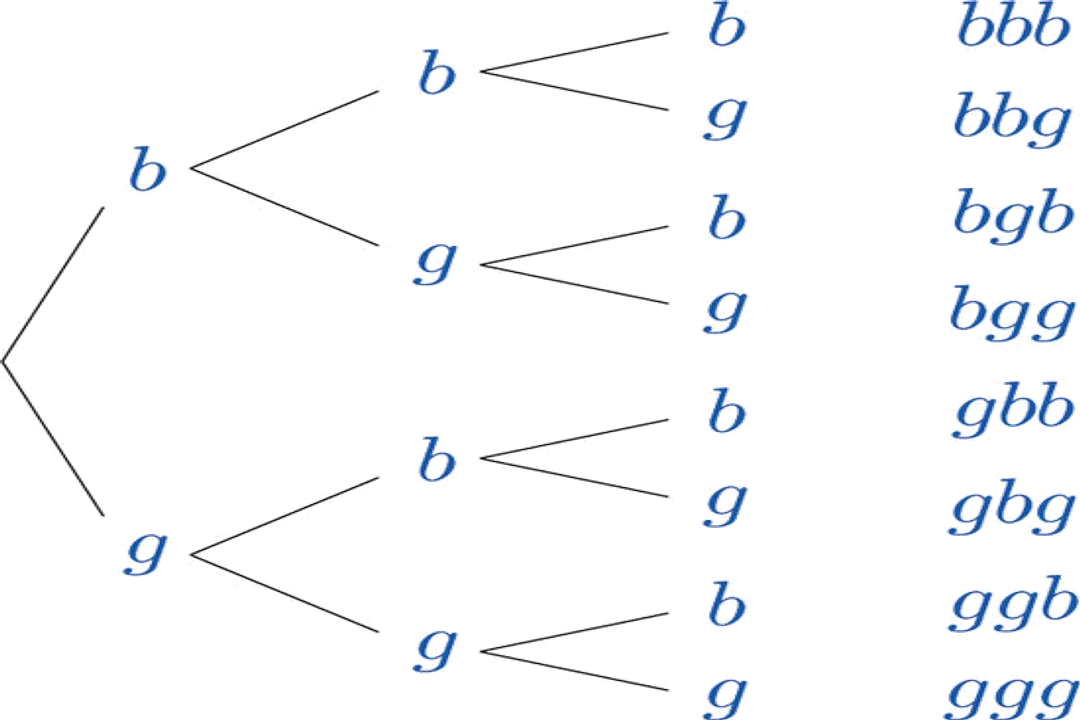
Another area where probability describes the boundaries of randomness is through the concept of complementary events. If $E$ is an event, its complement, $E^{c}$ , is the event that $E$ does not occur. ^[6] Since one of the two must happen, $P (E) + P (E^{c}) = 1$ , or $P (E^{c}) = 1 - P (E)$ . ^[6] This is often the easiest way to calculate the probability of a "complicated" event. For example, calculating the probability of getting at least one head in three coin flips directly involves calculating $P(\text{HHT}) + P(\text{HTH}) + P(\text{THH}) + P(\text{HHH})$ . It is far simpler to calculate the probability of the complementary event—getting zero heads, which is $P(\text{TTT}) = 1/8$ —and subtract that from one: $1 - 1 / 8 = 7 / 8$ . ^[1] This method shows probability describing a complex structure by leveraging the simplicity of its opposite.

# Putting It Into Practice

When applying this descriptive power, think about how you frame your question. If you are designing a warning system based on sensor readings, you aren't asking "Will the sensor trigger?" (a deterministic question); you are asking, "What is the probability that the sensor triggers, given that the actual condition is $X$ ?". ^[4] This moves the problem into the realm of conditional probability, where probability describes the accuracy and reliability of your measurement tool against the true random state of the world. ^[2]

A final, practical consideration is choosing the right model for the assignment of probabilities in the first place. If you are analyzing the spread of a rumor on a social network, you cannot easily assign equiprobable outcomes, nor is repeating the exact same network state feasible. In such cases, you move toward models that rely heavily on observed frequencies or Bayesian inference, where prior beliefs are constantly updated by new data. The description of randomness in this context is dynamic—the probability itself changes as new information about the system is gathered. ^[3] The mathematical description adapts from a static calculation (like a fair die roll) to a continuously evolving estimate, which is how probability describes the randomness inherent in learning and adaptation.

In summary, probability does not eliminate the element of chance; it frames it mathematically. It transforms the chaotic, unpredictable nature of an outcome into a quantifiable measure between 0 and 1 by defining the boundaries (the sample space), isolating the possibility (the event as a subset), and assigning a consistent, axiomatic measure to that isolation, whether through theoretical ratios, observed frequencies, or measures of belief. ^[5]^[6]