How does uncertainty arise in experiments?
Every scientific measurement, no matter how carefully performed, carries with it an element of doubt, a quantification of how well the result truly reflects the physical reality it intends to describe. This inherent quality of experimental results is what is known in the scientific community as uncertainty. [7][6] When a scientist reports a value, say a length of , they are not claiming absolute truth; rather, they are stating that the true value most likely lies within a specific range around . [2] Understanding how this uncertainty arises is fundamental to designing sound experiments, interpreting data correctly, and making meaningful scientific progress. [5][7] Uncertainty is essentially the range of values within which the true value of a measurement is believed to lie, giving context to the reported number. [2]
# Measurement Limits
Uncertainty is intrinsically linked to the act of measurement itself, stemming from the physical limitations of the tools and the process. [6] No measuring instrument, from a simple ruler to a sophisticated mass spectrometer, has infinite resolution or precision. [3] This concept separates precision, which relates to how close repeated measurements are to each other, from accuracy, which describes how close the measurement is to the true value. [4] An experiment might yield very precise results that are consistently wrong due to a systematic issue, while a less precise reading might accidentally land closer to the truth. [4]
The simplest way uncertainty manifests is through the apparatus used. For example, when reading a calibrated scale, the smallest division on the instrument dictates the lowest level of detail you can record. [9] If a digital balance reads to , the uncertainty is often taken to be or , depending on the standard practice for that instrument class. [2] This is often called instrumental uncertainty or reading uncertainty. [3] Even if you could perfectly reproduce the measurement an infinite number of times, this inherent resolution limit would remain. [6]
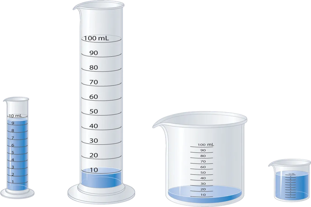
Beyond the physical device, the very act of observation can influence the result. In many experiments, the observer's skill in reading an instrument or controlling variables plays a part. [9] Consider reading the meniscus in a graduated cylinder: slight variations in eye level or judgment regarding the lowest point of the curve introduce variability that cannot be completely eliminated simply by using a better cylinder. [2] This human factor contributes a layer of uncertainty that must be accounted for, often through repeated measurements and statistical analysis. [2]
# Error Sources
The origins of experimental uncertainty are multifaceted, meaning they arise from various stages within the experimental procedure, not just the final reading. [2][9] We can generally group these origins into several categories, acknowledging that in real-world complex experiments, these sources often overlap and interact in non-trivial ways. [8]
# Apparatus and Instruments
The physical limitations of the measuring devices form the primary category of uncertainty contributors. [2][3] This includes issues like calibration drift, where an instrument's zero point shifts over time, or inherent imperfections in the scale markings themselves. [9] Even when an instrument is perfectly manufactured, thermal expansion or contraction due to ambient temperature fluctuations can subtly change its effective scale length, introducing an environmental factor directly into the instrumental uncertainty. [2] A well-designed experiment attempts to minimize these effects, for instance, by performing measurements in a temperature-controlled environment or by frequently recalibrating against known standards. [9]
# Environmental Factors
The surrounding conditions—temperature, pressure, humidity, vibrations, or electrical interference—can all influence a measurement without being the primary subject of the experiment. [2][9] For instance, measuring the resistance of a component is highly dependent on ambient temperature, as resistance changes with heat. [2] If the experimenter doesn't record or control the temperature, this variation becomes an unaccounted source of uncertainty in the resistance measurement. Recognizing this requires an awareness of the physics governing the measurement; an electronic measurement might be less affected by air currents than a sensitive balance measuring light powders, but both are susceptible to external influences. [9]
# Human Skill
The operator's technique is another critical area where uncertainty creeps in. [9] This isn't just about clumsiness; it involves the consistency of the technique. If one person times an event by starting a stopwatch when they see a light flash, and another starts when they hear the accompanying sound, the resulting time measurements will systematically differ due to reaction time variability. [2] When multiple people take measurements, the personal bias or reading style of each individual must be averaged out or tracked as a source of random variation. [2]
If we were to create a formal uncertainty budget for a simple chemical titration, we might see something like this structure:
| Source Category | Estimated Contribution (Estimated Standard Deviation, ) | Relative Impact |
|---|---|---|
| Volume dispensed (Burette reading) | High | |
| Mass weighed (Analytical Balance) | Medium | |
| Reaction endpoint detection (Visual) | () | High |
| Temperature fluctuation during reaction | Negligible for this reaction type | Low |
This simple exercise, budgeting the expected errors, is essential for determining which part of the procedure needs the most refinement for the next trial. [9]

# Error Types
The way uncertainty behaves and affects the final result is often categorized into two main types: random uncertainty and systematic uncertainty. [1][4] Distinguishing between them is crucial because they require different approaches to manage and minimize.
# Random Uncertainty
Random uncertainty, often referred to as random error, causes repeated measurements of the same quantity to fluctuate randomly around a central value. [1][4] This variation is unpredictable from one measurement to the next. Imagine tossing a dart at a target; some throws land slightly high, some slightly low, some left, some right, but they generally cluster around the bullseye. [2] This type of uncertainty arises from the uncontrollable fluctuations mentioned earlier—small changes in voltage, slight air currents, or minor differences in reaction time. [1] The key characteristic is that repeated measurements will help reduce the impact of random uncertainty on the final average. [2] Statistically, random uncertainty is handled using methods like calculating the standard deviation or standard error of the mean from multiple readings. [1][2]
# Systematic Uncertainty
In contrast, systematic uncertainty, or systematic error, consistently shifts the results in a particular direction away from the true value. [1][4] If the dart-throwing example had a consistent tailwind pushing every dart slightly to the right, that consistent bias would be the systematic error. In a lab setting, this could be caused by an improperly zeroed balance, a thermometer that consistently reads too high, or an observer who always starts the stopwatch slightly early due to a consistent physiological delay. [4][9] Because the error is consistent, taking more measurements will not reduce the systematic error; the average of a million biased readings will still be systematically wrong. [1][4] Identifying and correcting systematic uncertainty often requires careful calibration, comparison with established standards, or fundamentally redesigning the experimental method. [4][9]
# Combining and Reporting
When an experiment involves multiple measured quantities, each carrying its own uncertainty, the uncertainties must be combined to determine the total uncertainty of the final calculated result. [1] This process is known as uncertainty propagation. [1] The way these uncertainties are mathematically combined depends on whether the source uncertainties are treated as independent random variables or if a worst-case scenario analysis is preferred. [3]
For independent sources, a common method involves adding the squares of the individual uncertainties (often in quadrature), which is appropriate when the errors are random and uncorrelated. [1] However, if the calculation involves quantities that are highly dependent, or if a simpler, more conservative estimate is required, an alternative approach—the worst-case analysis—may be used, where uncertainties are simply added together linearly. [3] The choice between these methods reflects the scientist's confidence in the statistical nature of the errors versus the need for a definite upper bound on the potential error.
The final reported result must convey both the best estimate and the associated uncertainty clearly. [2] Typically, this is written in the form:
For example, reporting a mass as . [2] A crucial, though often overlooked, rule of thumb in reporting is that the uncertainty should generally be rounded to one, or occasionally two, significant figures, and the measured value should then be rounded to the same decimal place as the uncertainty. [2] Reporting is usually excessive and implies a false level of certainty about the uncertainty itself. [4]
# Hidden Assumptions
While the direct measurement process clearly generates random and systematic errors, uncertainty also arises from the model or assumptions used to interpret the data—a subtle but significant category that can sometimes be overlooked in basic lab courses. [8] When physicists or engineers attempt to model real-world behavior, they often simplify the system by neglecting secondary effects, such as air resistance in a projectile motion problem or the finite size of particles in a chemical reaction model. [8]
These neglected factors introduce an element of uncertainty that isn't captured by measuring the primary variables more precisely. For instance, one line of research suggests that in real-world experiments, physicists often fail to account for the uncertainty arising from the mismatch between a simplified theoretical model and the complex reality being observed. [8] If the underlying physical theory itself is an approximation—which is almost always the case when dealing with complex systems—then the resulting measurement is uncertain not just because the ruler was imperfect, but because the map being used to understand the territory is inherently incomplete. [7][8] A successful analysis must therefore consider not only the uncertainty in the data points themselves but also the uncertainty introduced by the theoretical interpretation applied to those points. [8] This moves the discussion from pure experimental error to the epistemology of scientific modeling.
When designing an experiment, especially for a novel or complex phenomenon, it is wise to treat the choice of analytical method as a primary source of uncertainty budgeting. If you know a specific variable has a known uncertainty , and your final calculated value depends on via , the resulting uncertainty will scale differently depending on the function . [1] For example, if you are calculating area () and has a $1%$ uncertainty, and has a $2%$ uncertainty, the resulting area uncertainty is not $1% + 2%$. It is found by combining the fractional uncertainties in quadrature (). [1] This non-additive, compounding behavior means that refining the measurement of the variable that has the greatest influence on the final result (the one whose uncertainty contributes most to the final summed square) yields the most significant improvement in the overall experimental confidence. [3] Focusing measurement refinement efforts on the weakest link in the mathematical chain is always the most effective strategy for reducing overall experimental uncertainty. [9]
Related Questions
#Citations
Experimental uncertainty analysis - Wikipedia
UNC Physics Lab Manual Uncertainty Guide
[PDF] Experimental Uncertainty
1.6: Uncertainties in Scientific Measurements - Chemistry LibreTexts
What is the uncertainty in an experiment? - Quora
Experimental Uncertainty - an overview | ScienceDirect Topics
What does uncertainty mean for scientists? - Sense about Science
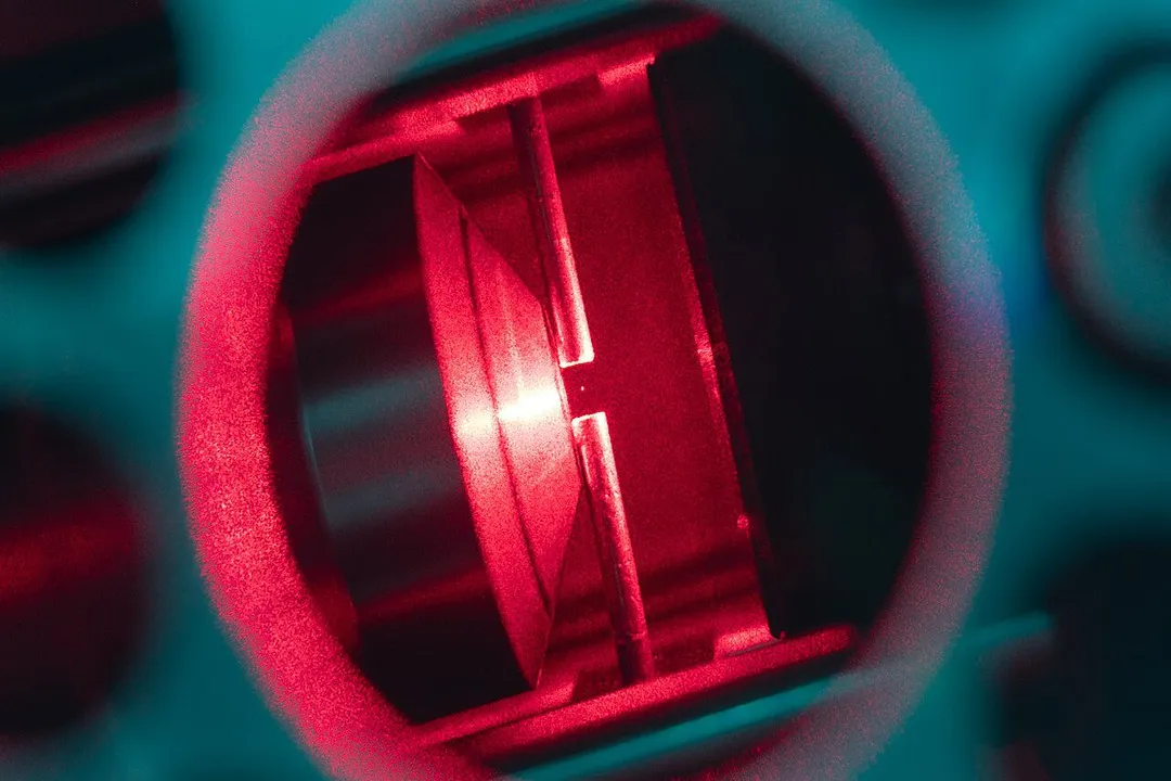
Physicists identify overlooked uncertainty in real-world experiments
[PDF] A Beginner's Guide to Uncertainty of Measurement