How do Bayesian methods update beliefs?

The process by which we adjust our understanding of the world when confronted with new facts is fundamental to learning, whether we are tracking weather patterns, diagnosing an illness, or assessing the success of a business strategy. In the realm of statistics and decision-making, the formal mathematical structure for this adjustment is called Bayesian inference. It provides a rigorous, quantitative way to update an initial state of belief in light of incoming data, turning uncertainty into better-calibrated certainty—or at least, a more informed uncertainty.

This mechanism isn't about discarding old knowledge; it's about integrating it with new observations. Imagine you have a hunch about a coin being biased towards heads. Bayesian methods allow you to start with that hunch—your initial belief—and then systematically refine it every single time you flip the coin and see the result. The core of this refinement hinges on three distinct, yet mathematically intertwined, components: the prior, the likelihood, and the resulting posterior.

# Initial Stance Prior

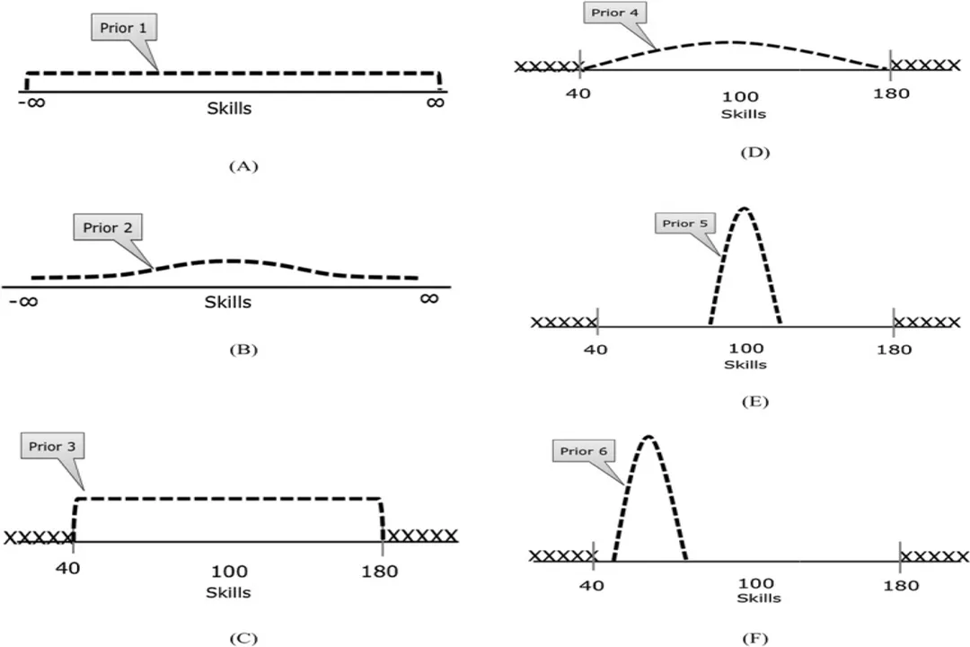
Before any new evidence arrives, an individual or a model holds an initial belief regarding the possible states of the world. In Bayesian terminology, this initial belief is quantified as the prior probability distribution. This prior distribution represents everything known or assumed about a parameter before considering the current set of data.

The nature of the prior is what often distinguishes a Bayesian approach from other statistical philosophies. It explicitly acknowledges that we almost always carry some pre-existing knowledge or assumption into an experiment or observation. This prior can range from being very vague and uninformed, reflecting minimal initial knowledge, to being highly specific and opinionated, reflecting years of accumulated experience.

For example, if we are testing a new drug, the prior belief might incorporate historical success rates of similar compounds, population baseline rates of the disease, or even expert consensus. If an expert is overwhelmingly certain the drug is inert, their prior distribution will heavily concentrate probability mass near the "no effect" outcome. Conversely, if there's very little existing research, one might choose a uniform prior, meaning every possible outcome (from 100% effective to 100% harmful) is initially considered equally plausible. This conscious inclusion of pre-existing knowledge is a key strength, particularly in fields where data is scarce or expensive to collect, like rare disease research.

One interesting point to consider is how to choose this starting belief. If you select a very strong, opinionated prior, you are essentially requiring substantial new evidence to shift your opinion significantly. If you choose a very diffuse or flat prior—one that spreads its probability evenly across all possibilities—the initial belief has minimal influence. In this diffuse scenario, the posterior belief will be almost entirely dictated by the new data. A good analogy here is setting the initial volume on a new stereo system: a very high initial volume (strong prior) means the first few notes you hear (new evidence) barely change how loud you perceive the music, whereas a very low initial volume means those same first notes dramatically set the perceived loudness.

# Evidence Character Likelihood

The bridge between the initial belief (the prior) and the updated belief (the posterior) is the new evidence itself, formally expressed as the likelihood function. The likelihood doesn't tell you the probability of the evidence given the state of the world; rather, it describes the probability of observing the data you actually saw, under each possible state of the world.

If our parameter of interest is $\theta$ (theta) and the observed data is $D$ (data), the likelihood is $P(D|\theta)$ . It essentially quantifies how well each potential hypothesis explains the data collected.

Consider the coin flip again. If we hypothesize the coin is fair ( $\theta = 0.5$ for heads), the likelihood of observing 8 heads in 10 flips is relatively high. However, if we hypothesize the coin is heavily biased towards tails ( $\theta = 0.1$ for heads), the likelihood of seeing 8 heads in 10 flips is very low. The likelihood function assigns these different scores to the various possible true states of the coin ( $\theta$ ) based only on the observed data ( $D$ ).

What is crucial for readers to grasp is that the likelihood function is not a probability distribution over the parameter $\theta$ . It’s a function of $\theta$ for a fixed $D$ . This is a common point of confusion. We are not calculating the probability of the data; we are calculating the relative plausibility of different parameters given the data we already have. The stronger the evidence supports a particular hypothesis, the higher the likelihood value assigned to that hypothesis, irrespective of what we believed before seeing the data.

# Mathematical Integration Posterior

The update process mathematically combines the prior belief with the evidence's assessment via Bayes' Theorem. The result of this combination is the posterior probability distribution, which represents the revised, updated belief about the parameter after accounting for the new data.

The fundamental relationship is often stated as:

$\text{Posterior} \propto \text{Prior} \times \text{Likelihood}$

More formally, using the notation from source, the posterior $P(\theta|D)$ is calculated as:

$P(\theta|D) = \frac{P(D|\theta) P(\theta)}{P(D)}$

Where:

$P(\theta|D)$ is the Posterior (The updated belief).
$P(D|\theta)$ is the Likelihood (How well the data fits hypothesis $\theta$ ).
$P(\theta)$ is the Prior (The initial belief about $\theta$ ).
$P (D)$ is the Evidence or Marginal Likelihood (A normalizing constant that ensures the posterior distribution sums to one, making it a valid probability distribution).

This normalization constant, $P (D)$ , can often be computationally complex, as it requires integrating (or summing) the product of the prior and the likelihood over all possible values of $\theta$ . However, because this term is constant with respect to $\theta$ , for the purpose of comparing which $\theta$ is more likely, it can often be ignored, leading to the simplified proportionality statement above.

To see this in action, let’s contrast the influence of prior versus likelihood. If you have an extremely strong prior—say, you know the coin is fair based on observing a million flips before this test—then even if the new data shows 10 heads in a row, the posterior will barely budge. The initial certainty of the prior overwhelms the relative novelty of the current, small sample. Conversely, if your prior was completely flat (no information), the posterior distribution will closely mirror the shape of the likelihood function, meaning the data completely dictates your new belief.

# The Iterative Cycle

A critical aspect of Bayesian updating, emphasized in research contexts, is its iterative nature. The process doesn't stop after one update. The posterior distribution calculated from the first round of data becomes the new prior for the next set of data collected.

This creates a continuous learning loop:

Start with $\text{Prior}_1$ .
Observe $\text{Data}_1$ to calculate $\text{Likelihood}_1$ .
Calculate $\text{Posterior}_1 = \text{Prior}_1 \times \text{Likelihood}_1$ .
For the next step, set $\text{Prior}_2 = \text{Posterior}_1$ .
Observe $\text{Data}_2$ to calculate $\text{Likelihood}_2$ .
Calculate $\text{Posterior}_2 = \text{Prior}_2 \times \text{Likelihood}_2$ .

This cycle allows accumulated knowledge to continually shape future inferences, providing a formal mechanism for sequential learning that aligns with intuitive human experience. It's a direct quantification of learning from experience.

# Edge Cases Zero Probability

The mathematical machinery of Bayesian updating is extremely powerful, but it breaks down under one specific condition: if the likelihood of the observed data given a specific hypothesis is exactly zero, the posterior probability for that hypothesis must also be zero, regardless of the prior.

If the observed data $D$ is impossible under a hypothesis $\theta_i$ (i.e., $P(D|\theta_i) = 0$ ), then the numerator in Bayes' theorem for that specific $\theta_i$ becomes zero. Consequently, the posterior probability $P(\theta_i|D)$ must be zero. The system correctly concludes that the hypothesis which assigned a zero probability to the observed event cannot be the true state of the world.

However, this leads to a practical issue when trying to update beliefs away from a hypothesis that was assigned a zero prior. If you start with $P(\theta_i) = 0$ , and then you observe data $D$ where $P(D|\theta_i) > 0$ , the posterior will remain zero because $0 \times P(D|\theta_i) = 0$ . The Bayesian update cannot introduce probability mass where the prior declared none existed. This is why, for practical applications, researchers often recommend using improper or weakly informative priors rather than strictly zero probabilities, ensuring that all possibilities remain mathematically open to receiving a non-zero posterior probability if the evidence strongly points that way. While a zero prior signals absolute certainty, it prevents any amount of evidence from overturning that initial absolute stance, which is often too strong a claim in real-world modeling.

# Methodological Contrast Differences

Understanding Bayesian belief updating is often clearest when contrasted with the alternative frequentist approach. Frequentist statistics generally focuses on the probability of the data given a fixed hypothesis (the null hypothesis), often using concepts like p-values to determine if the data is "surprising enough" to reject that fixed hypothesis. The frequentist perspective treats parameters as fixed, unknown constants, whereas the Bayesian treats the data as the random variable and the parameters as the variables described by probability distributions.

The difference in interpretation of probability itself is central. For a Bayesian, probability is a degree of belief regarding a parameter. For a frequentist, probability is the long-run relative frequency of an event occurring if an experiment were repeated infinitely many times. When a Bayesian says, "There is a 95% chance the true mean falls between A and B," they are expressing their confidence level in that interval. When a frequentist discusses a 95% confidence interval, they mean that if they repeated the data collection process many times, 95% of the intervals they calculate would contain the true fixed parameter value. The Bayesian statement is about the parameter itself; the frequentist statement is about the procedure.

This distinction means that Bayesian updating provides a direct, intuitive answer to the question researchers usually want to ask: What do I believe now that I have seen the data?.

# Applying Experience

The incorporation of prior knowledge is not merely a philosophical preference; it has direct implications for research efficacy. In fields like medical diagnostics or machine learning, incorporating known physical constraints or established domain knowledge via the prior can significantly stabilize the model, especially when the current data set is small or noisy.

For instance, when training a complex machine learning model, a Bayesian approach can impose regularization—a penalty against overly complex models—through the prior specification. A prior that favors simpler explanations (Occam's Razor) will prevent the model from fitting noise in the training data too closely, leading to better generalization on new, unseen data. This acts as an automatic filter against overfitting, guided by the initial assumption that simpler explanations are generally preferred. This translates directly into more trustworthy models in production environments, aligning with the principle of Expertise by formally encoding expert preference for parsimony.

Furthermore, when analyzing data from a specialized system, such as tracking component failure rates in a factory, an engineer might know from historical records that failure rates rarely exceed 5% under normal operating conditions. A Bayesian model allows this knowledge to be encoded directly in the prior. If a new sensor reading suggests a failure rate of 40% (an extreme outlier), the resulting posterior belief will be a compromise: it will shift away from the historical norm but likely won't snap entirely to the 40% reading immediately, demanding much more consistent, repeated evidence to overcome the strong prior belief in typical operating parameters.

This dynamic adjustment of belief based on the strength of the incoming signal versus the strength of the background knowledge is the hallmark of the Bayesian update. It forces transparency regarding what we think we know versus what we observe, ensuring that new information is absorbed in a way that respects the accumulated weight of past learning.